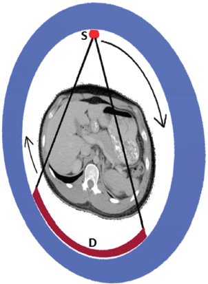
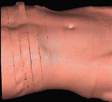
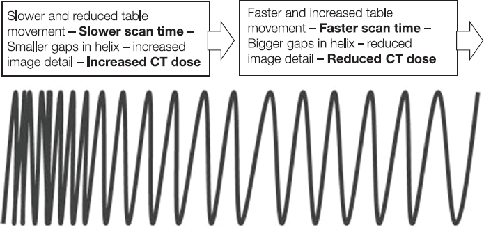
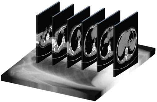
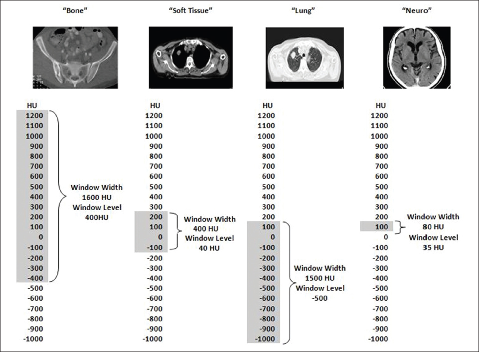
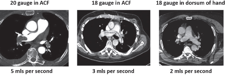
This book is intended to prepare the radiotherapy professional for CT interpretation of radiotherapy planning or image-guided radiotherapy scans. This introductory chapter provides some background details related to CT equipment and principles as well as potential problems and hints to aid image interpretation. All essential structures relevant to radiotherapy are described and depicted on labelled CT images covering the whole body. Each region of the body has its own chapter and within that chapter, various anatomical systems are described along with an overview of their CT anatomy on transverse sections. Three-dimensional images have been reconstructed from CT outlines and are presented to aid understanding of the relationships between structures. Labels and outlines are provided on real CT images alongside notes relating to image interpretation and tips for identifying structures. Within a region of the body each structure has its own identifying number, enabling them to be traced throughout the CT series with ease. The structure index contains a full list of these labels. After the different systems have been discussed, the full CT anatomy of the region is presented on labelled images alongside corresponding blank CT scans. Intracranial CT images are complemented with magnetic resonance (MR) and fused images where this represents common clinical practice. To aid the reader with this, there is a short introduction to some common MR imaging sequences and hints on image interpretation. The CT images in the book were all obtained using standard radiotherapy planning protocols and use immobilisation and positioning techniques that are similar to those found in radiotherapy. This distinguishes the book from other CT texts which utilise diagnostic views and patient positions. It must be borne in mind, however, that individual departments vary in positioning requirements almost as much as individual patients vary in anatomy. The reader is urged to use the images in this text to engender an understanding of how different structures relate to each other so that this knowledge can be applied to their own clinical practice. Each chapter concludes with a short self-test to consolidate and check learning. Answers to these can be found at the back of the book. The final chapter provides an overview of alternative CT imaging systems, including megavoltage CT, with some image interpretation. The emphasis of the book, however, remains on providing interpretation skills using standard kilovoltage CT images with a view to undertaking radiotherapy planning or Image-Guided Radiotherapy (IGRT) delivery. Medical imaging has utilised the mechanical movement of an x-ray source and imaging media to demonstrate layers or ‘slices’ in the human body since the early 1920s in the form of ‘stratigraphy’ (stratum – layer), later recognised as ‘tomography’ (tomos – Greek meaning section or slice). Further exploration of this concept, linked with reconstruction algorithms that can be traced back to theories by mathematician J.H. Radon in 1917 and evolution of the computer processing power necessary to process and reconstruct large amounts of data, led to the development of CT as we know it. Computerised Axial Tomography (CAT or CT) has revolutionised radiological diagnosis since its introduction into the clinical setting in 1972. CT was developed by several individuals, including Allan Cormack, Dr James Ambrose and Dr Robert Ledley. The most notable, however, was Sir Godfrey Hounsfield, a UK-born electrical and mechanical engineer. His name was immortalised in the name of the quantitative measurement scale used to evaluate CT images: the ‘Hounsfield Scale’. In 1971, Hounsfield and Ambrose conducted studies of the first clinical prototype on human and bovine brain specimens. Images from these studies demonstrated clear demarcation between tumour tissue and surrounding normal grey and white matter. Following this success, the first clinical examination of a real patient successfully demonstrated a dark cystic lesion in the brain and highlighted the clinical potential of CT. Following Dr Robert Ledley’s work in 1974, developing the first whole body scanner, a new era of medical imaging investigations began. CT’s ability to record very small differences in tissue contrast demonstrated the potential to demarcate disease process in relation to adjacent tissues. Given the potential for CT to image previously difficult areas such as intracranial tissues, it rapidly became the accepted imaging modality of choice for many clinical queries. As diagnostic confidence and imaging capabilities grew, it also became clear that radiotherapy accuracy could be greatly improved by utilising CT images in the tumour staging, treatment planning and more recently treatment verification processes. CT technology has evolved rapidly ever since, resulting in the current ‘third generation’ scanner, on which today’s CT equipment is based. Figure 1.2.1 Figure 1.2.1 illustrates the arrangement of the x-ray tube source (S) and detector array (D) in a typical modern scanner. A number of detector elements are arranged in an arc and rotate around the isocentre of the gantry simultaneously with the x-ray tube. Numbers of detector elements and rows vary between manufacturers; however the principle remains the same. The source emits a heterogeneous ‘fan’ beam of x-radiation that is collimated and filtered to specific body areas and types and aimed towards the patient in the centre of the gantry aperture. This beam is attenuated to differing extents depending on the tissue density, atomic number and electrons per gram of the tissue in its path. The detector array records the emergent attenuated beam, collecting data from multiple measurements as it rotates around the patient. The detectors contain scintillation crystals that emit visible light when irradiated. The intensity of this light is proportional to the attenuation of the original beam. The light is then converted into an electrical signal. The detector array is able to measure many thousands of signals with each rotation of the x-ray tube and these are then subjected to sampling and reconstruction. During image reconstruction, absorption values are assigned to each picture element (pixel) within each slice. A 2-dimensional image representation of the body area of that particular slice location is formed and typically shown on a 512 x[multi] 512 image matrix. This image resolution is sufficient for resolving sub mm changes in tissue contrast. The resolution of the whole CT system is dependent upon the size of each single detector, with some systems capable of resolving 0.5 x[multi] 0.5mm with similar sized detector elements. Spiral or ‘helical’ imaging can be achieved by simultaneously moving the table and patient though the scanner during image acquisition. The resulting spiral or helix of cross-sectional data is then produced with tiny gaps in it which are later interpolated by the reconstruction algorithm software. This is best imagined as resembling a spring viewed from the side. Figure 1.2.2 demonstrates the path of this spiral acquisition captured incidentally as the result of a patient coughing during a scan. The faster the table moves, the more the helix of the spring is pulled apart and the wider the gaps become, as shown in Figure 1.2.3. This impacts negatively on image detail, although patient dose and scan times are reduced. Figure 1.2.2 Figure 1.2.3 The ratio between the amount of table movement and tube rotation of the beam is called ‘pitch’ and can have a sizeable effect on both image quality and patient dose. If the table moves through the gantry slowly then the pitch will be lower, giving greater image detail but at the expense of increased patient x-ray dose. Multi-slice CT has been available since the early 1990s. Multi-slice scanners use an array of detector rows to acquire up to 64 ‘slices’ of data per tube rotation. This can be described as volumetric acquisition and has the benefit of greater tissue coverage together with considerably reduced scan times. At the time of publication, diagnostic systems with 128, 256 and even 320 multi-slice detector scanners are available and ever more complex cone beam reconstruction algorithms are being developed. Although it is possible to reconstruct images in the sagittal and coronal planes, most of the CT images in radiotherapy are traditionally displayed and viewed in the ‘axial’ or ‘transverse’ plane. Figure 1.3.1 illustrates a series of axial scans through the thorax. When displayed, each image is viewed caudally, i.e. from the patient’s feet upwards. When viewing each image, this must be taken into account. Thus the left side of the patient in Figure 1.3.2, which can be identified by the location of the heart, is on the right side of the image. Figure 1.3.1 Figure 1.3.2 also indicates that each slice is not merely a 2-dimensional image, but also has a measurement of depth. This depth is the slice thickness and is commonly manipulated at acquisition. Each image is also divided into a matrix of typically 512 x[multi] 512 pixels in the X and Y axes, although greatly simplified in the figure. Because each pixel also has depth, it has a volume in all three axes, and is called a volume element, or ‘voxel’. Ideally, to enable maximum image resolution and minimal distortion during post processing, each voxel should be cuboidal (or ‘isotropic’), for example, 0.5mm x 0.5mm x 0.5mm[multis]. During image reconstruction, each voxel is allocated a grey shade associated with specific tissue types within the cross-section; this is dependent upon the attenuation coefficient of the tissues. Figure 1.3.2 Ideally, for maximum image resolution, scanners should use the smallest slice thickness possible. This can present difficulties since imaging a whole chest or pelvis using 0.5mm slices would provide 400 to 500 images for analysis and planning. There are also patient dose and image noise implications to consider here; generally a thin slice requires a higher dose to reduce image noise to acceptable levels. Most radiotherapy planning scans therefore tend to utilise 3mm–5mm slice thickness as a compromise between image noise, patient dose and number of images produced. The detrimental effect of slice thickness on image resolution and hence upon the demarcation of structure boundaries is known as the partial volume effect. Figure 1.3.3 shows two slices of differing thickness; the image on the left is over 10mm, and the image on the right is 5mm thick. Figure 1.3.3 Attempting to identify a 5mm lymph node (marked in red) on the thick slice is fraught with difficulty, with the boundaries appearing less resolute and the overall attenuation value difficult to appreciate. This is because the slice thickness contains normal tissues above and below the node. By using thinner slices, the affected node will occupy the whole slice thickness and its borders and attenuation value will be more resolute and accurate. Any measurements or demarcation of borders will be more accurate on the thinner slice. The same applies for tortuous or rounded structures that may pass through part of the slice, where only part of the structure occupies the slice or other structures are superimposed. The value of using a range of images to aid interpretation cannot be emphasised enough. Figure 1.3.4 illustrates the thoracic aorta in red on all slices in the series. All such tubular structures running superiorly or inferiorly will be present on more than one image and can be traced above and below the slice being examined. This can help to distinguish between tubular and spherical structures such as lymph nodes. A similar technique can be adopted to assist with locating borders or determining centres of structures. It is important to view the images in this text not as isolated slices, but rather as part of a series and to interpret them in conjunction with adjacent slices. Figure 1.3.4 CT images are displayed using the convention of standard x-rays with the more dense ‘radio-opaque’ structures such as bone appearing white, and less dense ‘radiolucent’ structures appearing darker on the images. Sir Godfrey Hounsfield realised that he could plot specific attenuation units or values for each specific body tissue type falling within each pixel of the image. It would then be possible to calculate and plot any range of tissue densities found in a cross-section of human anatomy within each pixel of the image displayed. Thus an image of multiple tissue densities can be produced that is linked to reproducible measurable units of attenuation. These units are aptly named ‘Hounsfield Units’ (HU), and follow a scale centred on water, where water measures 0HU. Tissues of greater density or attenuation value have positive values, and densities of lower attenuation are given negative values. CT systems are capable of measuring an approximate range from +3000HU to -1000, although in practice the scale maximum is set at +1000HU. Figure 1.3.5 demonstrates the Hounsfield Scale, with further detailed breakdown of HU between +100HU and -5HU illustrating the range of units for soft tissues and fluid. This diagram indicates one of the inherent problems experienced when differentiating between soft tissue types with similar HU values. In order to view all the attenuation values, at least 2000 shades of grey (from black to white) would be required. Today’s monitors are capable of displaying over 250 grey tones, but the human eye can only distinguish between a maximum of 50–100 dependent upon ambient conditions. It is clear here then that small changes in tissue density would be missed if over 250 shades of grey were used. This failure to detect subtle changes in represented tissue density would lead to poor diagnosis and demarcation of structures, particularly between tissues possessing similar densities. By selecting the proportion of relevant HUs we wish to display, we can greatly improve the possibility of distinguishing between differing tissues. This method of image manipulation is called grey level mapping, or ‘windowing’. Windowing reflects the method used in CT to maximise image contrast by choosing a median HU value called the ‘Level’ and a range of HU either side of this called the ‘Width’. A wide window displays a large range of HU, and is useful for visualisation of detail across a wide range of tissue densities, such as in bones. By looking at the HU in Figure 1.3.5, it is evident that bone HU values range from approximately 200HU to 1000HU; for optimal image detail all these HU must be displayed. At the other extreme, when identifying tissue types where the HU variation is much narrower, the width must be reduced. For intracranial imaging, normal grey and white matter ranges from approx 22HU to 42HU, with cerebrospinal fluid measuring approximately 0HU. Thus a much narrower window must be selected to identify normal and abnormal intracranial anatomy. Figure 1.3.5 Figure 1.3.6 Once the appropriate width of tissue HUs has been chosen, the central point of this width or level on the Hounsfield Scale needs to be selected. The window level to distinguish bony detail would therefore be at the central point or mean of the HU value of normal bone (approximately 400HU). Figure 1.3.6 indicates the most widely used window widths and levels for radiotherapy applications. Diagnostic colleagues may also utilise more specific windowing widths and levels for appreciation of other tissues such as the liver. It is important to appreciate that tissue types with Hounsfield Units falling outside the selected width and level will be either white or black, and thus lacking in detail. If visual analysis is difficult due to ambient viewing conditions or inexperience, it is possible to acquire accurate digital measurements for each tissue type HU within the slice. Software on all scanners is configured to perform this function, and by comparing the digital measurements with HU guides (such as Figure 1.3.5) tissue types can be established. It is evident from Figure 1.3.5 that there are some tissue types that fall within a very narrow band of HU values, giving them a very similar appearance on images. If these tissues are in close proximity to one another this similarity can make it impossible to distinguish between structures and demarcate borders. In radiotherapy, this is a particular challenge in centrally located disease where there may be lymph node involvement with a lack of discernible border between blood vessels, the gastrointestinal tract and possible lymphadenopathy. These difficulties are common in centrally located bronchial tumours, lymphomas or pelvic tumours where regional iliac lymph chains may be affected. In these cases, introduction of a contrast agent with a substantially different HU value can highlight different structures, usually in the circulatory or digestive system. The following section outlines the key advantages and indications related to contrast agent usage; the reader is also directed to the CT safety section (1.5.2) for important information concerning safe use of contrast agents. Intravenous contrast The presence of iodine in blood plasma or target organ increases density for a limited time period during CT acquisition. Delivery of IV contrast agent is via an 18 gauge (green) or 20 gauge (pink) cannula (peripheral vascular access device (PVDA)), sited most commonly in the basilic vein ante-cubital fossa (ACF). Optimal visualisation of intraluminal vascular detail is dependent on injection delivery rate, volume and type of IV contrast utilised, and relies upon peak enhancement of the vasculature at the time of CT acquisition. The choice of peripheral venous access site and size of PVDA play a crucial role in achieving peak contrast enhancement at scan acquisition. A 20 gauge pink PVDA will permit the injection of a tight bolus of contrast media at between 4 and 5mls per second, optimising peak enhancement of contrast agent in the pulmonary, carotid and coronary arteries at the time of scan. Slower injection rates lead to reduced volumes of contrast media present within the vasculature at the time of scan acquisition, giving rise to reduced differential between iodine/plasma levels and potential thrombus/luminal abnormalities. Figure 1.3.7

1.1Purpose of the book
1.2CT Principles and Equipment
1.2.1CT Development
1.2.2Basic CT Principles
1.2.3Spiral CT
1.2.4Multi-slice CT
1.3CT Interpretation
1.3.1Viewing axial images
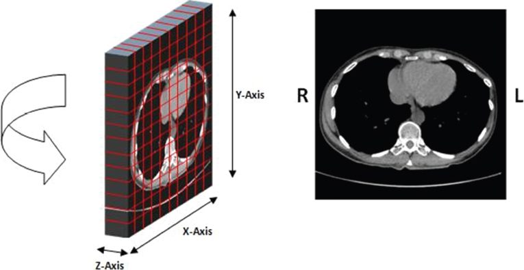
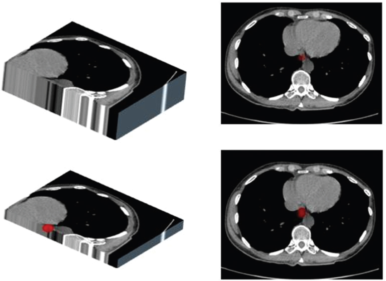
1.3.2Slice thickness and ‘partial volume’ effect
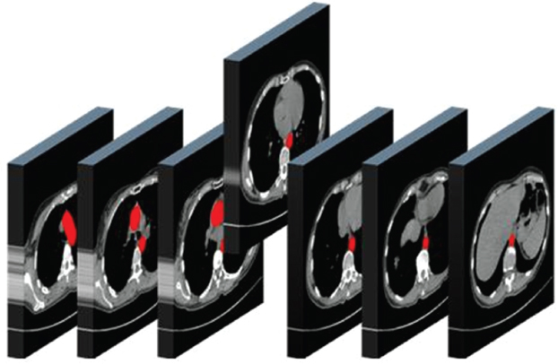
1.3.3Viewing the whole series of images
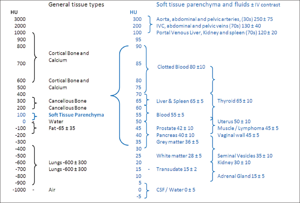
1.3.4Using Hounsfield Units
1.3.5Using contrast
![]()
Stay updated, free articles. Join our Telegram channel


Full access? Get Clinical Tree


