Liver Perfusion Imaging with MR
Maxime Ronot, MD, PhD
Benjamin Leporq, PhD
Simon A. Lambert, PhD
Jean-Luc Daire, PhD
Bernard E. Van Beers, MD, PhD,
Valérie Vilgrain, MD, PhD
▪ Introduction
The liver is a large, highly vascularized, subcutaneous solid organ that is easily accessible with various imaging techniques, including magnetic resonance imaging (MRI). Perfusion imaging provides information about tissue microcirculation or the movement of water and solutes at levels far below the spatial resolution of imaging techniques. Thus, perfusion imaging is not the dynamic qualitative analysis commonly obtained with tissue enhancement, but a quantitative extraction of physiologic perfusion parameters of the liver. MR perfusion imaging of the liver is based on the same principles as those used in other organs: the injection of a gadolinium chelate contrast medium (called a tracer) and acquisition by rapid temporal sampling of signal-intensity/time curves that provide information on variations in tracer concentrations over time. The physiologic parameters are extracted from these curves by adjusting them to mathematical perfusion models. Because of certain features of the liver, perfusion imaging is more challenging than in other organs. Indeed, the liver is a large, mobile organ that deforms with respiratory movements and has a dual vascular supply through the hepatic artery and the portal vein. In addition, the sinusoidal capillaries are fenestrated in the normal liver so the tracer readily diffuses from them.
Liver perfusion imaging is based on the hypothesis that local or diffuse pathologic processes result in measurable changes in perfusion parameters. Information is obtained about the presence or progression of these pathologic processes by quantifying these changes. Perfusion imaging is indicated in the liver for two main conditions: (a) Malignant liver tumors, in particular hepatocellular carcinoma (HCC) and liver metastases; and (b) the investigation of chronic liver diseases. Imaging already plays an important role in these two fields because imaging techniques (mainly CT and MRI) provide highly accurate qualitative data for the detection and characterization of liver lesions, treatment assessment, and patient follow-up. Therefore, the benefits of perfusion imaging must be evaluated not to replace existing techniques but as a complementary tool to adapt patient management or provide an earlier and more reproducible evaluation.
This chapter describes the bases and limitations of the different MR perfusion imaging techniques of the liver and discusses the clinical indications for liver perfusion studies.
▪ The Vascular Physiology of the Liver
The liver has a dual blood supply and receives approximately 25% of its blood from the hepatic artery and the remaining 75% from the portal vein. There is no hepatic capillary network per se. It is replaced by fenestrated sinusoids. These two afferent vascular systems communicate through transsinusoidal and transvasal communications as well as the peribiliary plexuses. One of the fundamental adaptive mechanisms involved in vascular abnormalities of the liver is the presence of an arterioportal balance called the “hepatic buffer response” characterized by a compensatory increase in arterial blood supply when portal supply decreases, although the reverse does not occur.1
▪ MR Imaging Techniques
In 1999, Scharf et al.2 found a significant correlation between MRI and thermal dilution probe flow measurements in pigs using 1.0 T T1-weighted (T1W) sequences. Many MRI techniques can be used for analysis of the microcirculation, including arterial spin labeling (ASL)3 in which the circulating blood is magnetically labeled, and the more recent combination of ASL with diffusion.4 In blood oxygen level dependency (BOLD) imaging,5 the ratio of oxygenated hemoglobin and paramagnetic deoxygenated hemoglobin can be used to obtain an indirect analysis of the oxygen supply in tissue. The two latter techniques are not used in the liver and will not be discussed.
The most common approach is a kinetic analysis following injection of a bolus of contrast material through tissue. When negative enhancement is evaluated (signal drop due to the effects induced by the first-pass of a bolus of concentrated contrast agent in T2/T2*-weighted MRI sequences), the technique is called dynamic susceptibility contrast-MRI (DSC-MRI). Although this was one of the first techniques to be investigated, today it is essentially indicated in brain perfusion analysis. Indeed, strictly speaking, DSCMRI is not used to investigate capillary leakage, and its analysis theoretically implies the presence of an intact blood-organ barrier, impermeable to contrast agents. Thus, it is not used in the liver and will not be discussed in this chapter. The evaluation of positive enhancement (T1 effect of the contrast agent) is called
“dynamic contrast-enhanced-imaging” or DCE imaging. This is the most common technique used in the liver, and the rest of the chapter describes it in detail. Besides conventional DCE sequences, sequences that measure molecular diffusion (diffusion-weighted MRI) are also influenced by microperfusion. This notion, which is called the IVIM model (intravoxel incoherent motion), was initially developed by Le Bihan et al.6 to quantitatively measure the microscopic movements that contribute to the diffusion MR signal. In biologic tissue, these movements are mainly due to the molecular diffusion of water and the microcirculation of blood in the capillary network (perfusion). Le Bihan et al. developed the notion that water circulating in randomly oriented capillaries (at a voxel level) imitates random motion (“pseudodiffusion”). This attenuates the diffusion MRI signal, which depends upon the speed of the circulating blood and the vascular architecture. Like true molecular diffusion, the effect of pseudodiffusion on signal attenuation depends on the b value. The amount of signal attenuation that occurs from pseudodiffusion, however, is greater than molecular diffusion in tissue, and, as a result, the relative contribution to the diffusion-weighted signal is only significant at very low b values, theoretically allowing diffusion and microperfusion components to be separated.
“dynamic contrast-enhanced-imaging” or DCE imaging. This is the most common technique used in the liver, and the rest of the chapter describes it in detail. Besides conventional DCE sequences, sequences that measure molecular diffusion (diffusion-weighted MRI) are also influenced by microperfusion. This notion, which is called the IVIM model (intravoxel incoherent motion), was initially developed by Le Bihan et al.6 to quantitatively measure the microscopic movements that contribute to the diffusion MR signal. In biologic tissue, these movements are mainly due to the molecular diffusion of water and the microcirculation of blood in the capillary network (perfusion). Le Bihan et al. developed the notion that water circulating in randomly oriented capillaries (at a voxel level) imitates random motion (“pseudodiffusion”). This attenuates the diffusion MRI signal, which depends upon the speed of the circulating blood and the vascular architecture. Like true molecular diffusion, the effect of pseudodiffusion on signal attenuation depends on the b value. The amount of signal attenuation that occurs from pseudodiffusion, however, is greater than molecular diffusion in tissue, and, as a result, the relative contribution to the diffusion-weighted signal is only significant at very low b values, theoretically allowing diffusion and microperfusion components to be separated.
Dynamic Contrast-Enhanced MR Imaging
Contrast-enhanced MRI corresponds to the acquisition of images of the liver during the arterial, portal venous, and delayed phases following a bolus injection of a gadolinium chelate (0.2 mmol/kg followed by 20 mL saline flush at 3 mL/s). When a hepatocytespecific contrast agent such as gadoxetic acid (Gd-EOB-DTPA) is used, a hepatobiliary phase (20 minutes) is added to the dynamic phase to assess intracellular retention of the contrast agent. To perform DCE-MRI, sequences can be accelerated (or time resolved) to obtain multiple dynamic scans.7 DCE-MRI is usually performed with diffusible agents. High temporal resolution is needed because the concentration changes rapidly in the arterial vessels during the first pass and correct sampling of the concentration versus time curves is essential. A temporal resolution less than 3 seconds is usually recommended, but a resolution of 1 second may be needed to visualize aortic peak enhancement. It is difficult to obtain this time resolution with whole-liver 3D MRI. Moreover, the relationship between signal intensity and tracer concentrations is not linear with MRI, unlike CT scan, in which the tracer concentration curve over time is proportional to changes in attenuation measured in Hounsfield units. A common DCE-MRI protocol is coronal 3D T1W fast gradient echo such as FLASH (TR = 2.7 milliseconds, TE = 0.9 millisecond, flip angle = 18 degrees, partition thickness = 8 mm, temporal resolution = 2 seconds for a 10 slice slab). A total of 180 consecutive measurements will be obtained. Precontrast images are obtained with two different flip angles (4 and 18 degrees) to analyze T1 values. The contrast will be injected after completion of first noncontrast measurement. In 3D acquisition, the first and the last couple slices will be excluded from analysis to remove wrap artifacts.
Nonlinear Relationship between Signal Intensity and Tracer Concentration
The nonlinearity of signal intensity and tracer concentrations can be seen when looking at the pulse sequence used for DCE-MRI. Indeed, these sequences are very sensitive to signal saturation and flow resulting in nonlinearity. Gadolinium concentration can be calculated from differences in T1 relaxation time before and after contrast. Precontrast T1 can be calculated from two or more sets of precontrast images using different flip angles, and postcontrast T1 values can be obtained from postcontrast and precontrast series with different flip angles.
Signal Saturation
Traditionally, the pulse sequences used were based on a spoiled gradient echo scheme with a short echo time (<1 millisecond) to decrease the T2* effect and a short repetition time (<4 to 5 milliseconds) to keep a suitable temporal resolution. The sequence dynamic is poor in this case, and depends upon the flip angle that significantly influences the linearity between T1 (thus concentration) and signal intensity (Fig. 27-1). The signal for long T1 structures—such as the liver—can be maintained with a small flip angle (<10 degrees) before enhancement, while the signal saturates during the enhancement peak of short T1 structures, such as the aorta.
Indeed, during these sequences the spins receive repeated RF pulses and there is not enough repetition time for longitudinal recovery of magnetization. As a result, spin magnetic moments are likely to be in the spin down direction and enter in a saturated state inducing signal saturation. This effect is emphasized by a large flip angle, by a short repetition time, and by the number of impulses. For conventional cartesian acquisitions, the k-space profile order is linear and the central lines are acquired halfway through the acquisition, after a significant number of repetitions (depending on the spatial resolution). Since this part of the k-space encodes for contrast, the saturation effect is predominant and may artificially erase contrast enhancement. This is very important to consider for quantitative perfusion imaging. A centric low-to-high profile may also be used (Fig. 27-2). This allows central lines of the k-space to be read first, limiting saturation as well as providing a better signal-tonoise ratio. A reverse linear profile is also an alternative with partial Fourier imaging in the phase direction.
Sensitivity to Flow
It is also very important to understand that the pulse sequences used for DCE-MRI are highly flow sensitive and influenced by a flow-related enhancement effect and entry slice phenomena. During the flow-related enhancement effect, the RF pulse selectively excites a volume while the rephasing gradient is applied to the entire body. Therefore, a flowing spin receiving an excitation pulse will be rephased regardless of its position. A stationary spin receives repeated RF pulses that tend to saturate, so flowing spin appears to have a higher signal. This phenomenon is emphasized by short
repetition times and short echo times as well as when the thickness of slice increases; thus it is predominant in DCE-MRI.
repetition times and short echo times as well as when the thickness of slice increases; thus it is predominant in DCE-MRI.
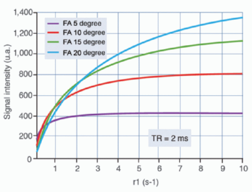 Figure 27-1. Simulation representing the signal intensity according to the longitudinal relaxation rate (1/T1) for different flip angles and with an ultrashort repetition time (2 milliseconds). These simulations illustrate the nonlinearity of the sequence according to r1 and the strong effect of flip angle on the dynamic. With small flip angles, dynamic is poor and saturation appears for short T1 structures. |
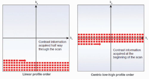 Figure 27-2. Scheme illustrating two k-space filling according to a linear profile order and to a centric low-high profile order. |
During the slice entry effect, the magnetic moments of spins receiving repeated RF pulses are usually oriented in the spin-down direction since the repetition time is not long enough for longitudinal recovery of magnetization in the tissue where the spin resides. Spins that have not received repeated RF pulses are called “fresh” since their magnetic moment is mainly orientated in the spin-up direction. Thus, flowing spins, perpendicular to the slice, enter it “fresh” because they have not received repeated RF pulses, and they produce a higher signal than do stationary spins in the slice. This effect increases with velocity and countercurrent flows and is therefore very strong in large vessels such as the abdominal aorta and the main portal trunk.
The Nonlinear Relationship between Signal Intensity and Concentration
The relationship between the signal and tracer concentrations need not necessarily be linear but must be clear. One simple solution to prevent the above-mentioned effects would be “spatial presaturation,” which delivers a selective 90-degree pulse to a volume outside the field of view (FOV) or the use of a nonselective preparation pulse in the sequence.
Several strategies have been suggested to manage the nonlinear relationship between signal intensity and gadolinium agent concentrations. First, precalibration can be performed by preparing scans with different tracer concentrations.8,9 Although the results of this method are accurate, it is complicated to perform in clinical practice and may decrease reproducibility. Autocalibration is another alternative. This involves computing a T1 precontrast map with a multiple flip angle acquisition corresponding to a dynamic acquisition flip angle in order to derive the T1 postinjection. Finally, plasma concentrations can be determined based on knowledge of tracer r1 relaxivity. Indeed, although the longitudinal relaxation rate and the signal intensity do not vary linearly, the relationship between r1 and the contrast agent concentration is linear based on:
where R1post is the postcontrast longitudinal relaxation rate, R1pre is the precontrast longitudinal relaxation rate, r1 is the longitudinal relaxivity of the contrast agent, and C is its concentration. This equation assumes that the relaxivity of the contrast agent is the same in blood and tissue, and that exchanges of water between intravascular, extravascular, and intracellular spaces are fast.8
However, this method is sensitive to the nonuniformity of the transmitted B1 field as well as to the nonlinearity of the RF transmission chain that affects small flip angles in particular, especially with 2D acquisitions. This can be corrected using a B1 map. Moreover, these measurements should be obtained from 3D images because of the imperfect slice selection profile of 2D images. Finally, a simple linear relationship between signal intensity and contrast agent concentrations is often assumed. In this case, low contrast agent concentrations (0.025 mmol/kg) and/or lower injection rates should be used to avoid saturation of signal enhancement at high concentrations. The pulse sequence setting should also be carefully performed to minimize the nonlinearity effect. While most groups use conventional gadolinium chelates, recent studies have reported the use of specific hepatobiliary contrast agents with similar results.10
▪ The Technical Challenges of Liver Perfusion Analysis
Pandharipande et al.11 published a list of requirements for an ideal liver perfusion analysis:
Accurate quantification of overall or regional arterial and portal perfusion to assess focal or diffuse abnormalities
High spatial resolution to examine small lesions
High temporal resolution to correctly identify the kinetic properties of tracers, which may differ within tissue lesions
Accurate quantitative analysis by measuring concentrations of reliable tracers
Robust modeling of the physiology of liver perfusion
“Whole-liver” imaging
Compatibility with morphologic imaging modalities so that complementary perfusion studies can be performed with more conventional studies
This list highlights the difficulties of studying the liver. Besides the well-known limitations of MRI—such as accessibility and cost—liver perfusion imaging involves several specific challenges and limitations that result in significant variability of results, in particular, the difficulty of accurately modeling liver perfusion and the size and mobility of this organ.
Liver Perfusion Modeling
Perfusion analysis relies entirely on the analysis of tracer concentration-time curves whose shape depends on tissue perfusion parameters, the characteristics of the tracer bolus (volume,
injection rate), and the patient’s cardiovascular parameters (cardiac output, ejection fraction).
injection rate), and the patient’s cardiovascular parameters (cardiac output, ejection fraction).
There are two main mathematical approaches to studying liver perfusion (Fig. 27-3): The semiquantitative approach based on the shape of the signal intensity/time curves (descriptive methods) and the quantitative approach based on concentration-time curves using a perfusion model (pharmacokinetic approach).
Descriptive methods of signal intensity/time curves are not based on any physiologic hypothesis (free models). Computers can be used to automate shape recognition of the enhancement process to create enhancement maps and detect areas of interest (e.g., hypervascular areas). Several descriptive or “heuristic” parameters can be analyzed from the tissue enhancement curve, such as the slope of enhancement (maximum slope), maximum enhancement (peak height) expressed in a percentage and the time to peak. Hepatic perfusion index (HPI) is another semiquantitative parameter that describes the relative contribution of arterial flow or portal flow to the total (arterial + portal) liver perfusion and can be easily calculated using different imaging techniques. HPI reflects the amount of arterial supply to the tumor or liver and its calculation does not require AIF or modeling. The time to peak in the splenic enhancement curve is used to distinguish between the arterial and portal venous phases of the liver. For perfusion analysis, the radiologist will place ROIs in the aorta, main portal vein, normal liver parenchyma, lesion, and the spleen. Liver arterial or venous perfusion will be estimated by the maximum slope in the liver enhancement curve before or after the splenic peak, respectively, divided by the peak aortic enhancement.
It should be noted that descriptive parameters may be affected by the instability of curves due to liver and vessel displacement. The area under the curve (AUC), that is, the integral under the enhancement curve, is a common parameter, because it is less affected by noise and does not require a mathematical model.12 Finally, raw semiquantitative evaluation does not take into account the intraarterial kinetics of the contrast agent, which may differ significantly among patients depending on the injection protocol (volume, concentration, injection rate, etc.) and physiologic conditions (respiration, cardiac output). They can be corrected by comparing results to those of a reference tissue such as muscle tissue or a nonpathologic portion of the liver. Correction is performed by calculating ratios to obtain relative parameters. These simple approaches may be very sensitive to the quality of the acquisitions.
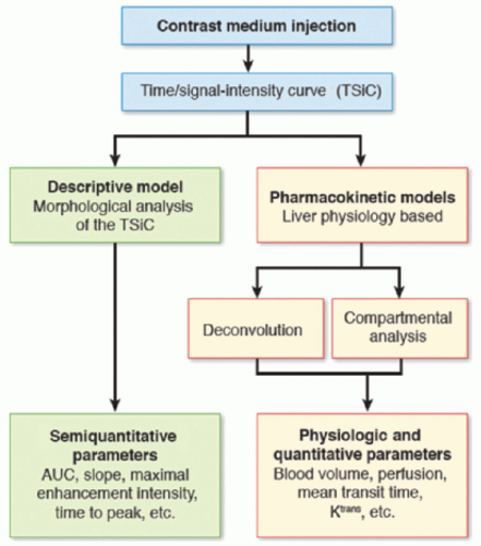 Figure 27-3. Schematic representation of the different models used in liver perfusion imaging analysis. (AUC, area under the curve.) |
Pharmacokinetic models incorporate specific characteristics of liver perfusion. These models are based on the relationship between arterial input alone (in tumors for instance) and arterial and portal input (in diffuse liver disease), obtained from the enhancement curve of the afferent blood vessels. Deconvolution algorithms and compartmental models13,14 belong to this category. The latter are based on the assumption that contrast enhancement is present in several hepatic compartments mixed in uniform concentrations, that flow between compartments is linear (passive exchange only) and that the parameters describing compartments do not vary during data acquisition. The parameters being studied are then extracted, depending on the models, which vary in the number of compartments and afferent blood vessels. Normal liver tissue can be considered a single compartment since there is free passage of contrast between the sinusoid (intravascular compartment) and the space of Disse (extravascular component). Therefore, in normal liver tissue, parameters related to extravasation of contrast into the interstitial space (such as permeability-surface area product) are not measurable. In contrast, in cirrhosis, the sinusoids become capillary-like and increased deposition of collagen in the space of Disse separates the intravascular from the extravascular space and contrast kinetics in the interstitial space become measurable.13
The T1 relaxation rate (i.e., tracer concentration) versus time curves can be analyzed with a dual-input model in the liver because it has two vascular inputs. The dual-input, single-compartmental model validated by Materne et al.8 is often used. The arterial, portal venous, and total liver blood transfer constants K1a, K1p, and K1t, respectively (mL/min/100 mL) can be assessed with this model as well as the distribution volume (DV) (%) and the mean transit time (MTT) (s) (1/k2).
K1 represents total perfusion and permeability as follows:
where F is the perfusion and E is the extraction fraction, varying between 0 and 1. When permeability is high as in the normal liver— which has fenestrated sinusoids—the extraction fraction equals 1 and K1 represents perfusion. If permeability is low, K1 represents PS, the permeability-surface area product.15 To measure vascular input, an ROI is placed in the portal vein and the abdominal aorta to be used as a surrogate for hepatic arterial blood supply. For dual-input one-compartment models, it is mandatory to include two delays (arterial and portal) in the model to take into account the temporal offset between central compartment input and measured input from arterial and portal ROIs.9 Nevertheless, the addition of two fitting parameters in the model increases the degree of freedom involving local minima problems. Thus, some groups have proposed to fix the delays manually. While arterial delay can be simply estimated from a curve analysis, manual estimation of portal delay is tricky. To address this issue, some groups have assumed the equality between portal and arterial delays. This approach has two main limitations. First, since delays spatially vary (depending on the ROI location), this approach is restricted to small ROI analysis and unsuited for mapping. Secondly, the assumption of equality between arterial and portal delays is very approximate since the delays are dependent on the blood flows. An alternative could be to include both delays in the model and to use an advanced optimization procedures such as
multistart approaches for the fitting procedure. Classically, the modeling is achieved using solvers based on a nonlinear least square fit. These methods are prone to local minima problems mainly linked at the choice of starting values. Multistart methods, by repeating the fitting procedure with pseudorandom starting values reinitialized each time, uncorrelate the fitting procedure from the choice of starting values, and reduce local minima problem. The main limitation of these approaches is the computing time increase due to repetition of fitting procedure.
multistart approaches for the fitting procedure. Classically, the modeling is achieved using solvers based on a nonlinear least square fit. These methods are prone to local minima problems mainly linked at the choice of starting values. Multistart methods, by repeating the fitting procedure with pseudorandom starting values reinitialized each time, uncorrelate the fitting procedure from the choice of starting values, and reduce local minima problem. The main limitation of these approaches is the computing time increase due to repetition of fitting procedure.
In contrast to the liver parenchyma, primary and secondary tumors of the liver, except very early stage, have only arterial but no portal venous input.16 Therefore, the perfusion of hepatic tumors can be analyzed with single-input rather than dual-input models. There are several single-input models available to assess tumors. The most frequently used models include a simple single-compartmental model, known as the Tofts (or Kety) model in which Ktrans (=K1) and the extravascular extracellular volume (ve = vd) are assessed; the extended Tofts (or extended Kety) model (which takes into account the contribution of the tracer in the vascular space), in which Ktrans, ve, and plasma volume (vp) are assessed; and the St. Lawrence and Lee model, which is a distributed-parameter model with four free parameters: tissue plasma flow (F), the extraction fraction (E), the extravascular extracellular volume (ve), and the mean capillary transit time (MTT). The capillary permeability-surface area product (PS) and the plasma volume (vp) can be derived from these parameters.17 Although a consensus conference has been published,18 there is still no consensus about the best model. The distributed St. Lawrence and Lee model is more physiologic with a separate calculation for perfusion and permeability, but is less precise than are the compartmental models due to the interdependency of the free parameters and their sensitivity to initial values. The problem of the uniqueness of the solutions may be even more complex when a dual-input distributed model is used, as recently proposed.19 Thus, the extended Tofts model may be a good compromise to estimate perfusion parameters in tumors because neither data interpolation nor supervised fitting is required.18
The transfer constant Ktrans and the extravascular extracellular volume ve are the recommended primary and secondary end points, respectively, of perfusion measurements.18 Both variables should be obtained, although the reproducibility of ve is better than that of Ktrans (repeatability coefficient of 30% for ve vs. 100% for Ktrans), and it can be used to assess vascular permeability by determining the volume accessible to contrast agents with different molecular wei ghts.17,20,21 However, the data obtained are not independent from the model or the software package used for analysis. This has been clearly demonstrated with CT perfusion studies.22
The Liver Is a Mobile Organ
Radiographic studies using fixed landmarks, radioscopy, and even CT23 have shown that the liver is an organ that moves considerably during breathing, shifting approximately 20 mm along its craniocaudal axis, 10 mm along its anteroposterior axis, and 5 mm laterally.
Related posts:
 Vascular Anatomy and Microanatomy
 CT and MR Contrast-Enhanced Tissue Perfusion Imaging: Basic Methodology, Postprocessing, Reliability Testing
 Clinical Applications of ASL Brain Perfusion Imaging
 Perfusion CT Imaging in Oncology
 Ultrasound Perfusion Imaging: Techniques and Analytical Methods
 Contrast-Enhanced Ultrasound: Clinical Applications
Stay updated, free articles. Join our Telegram channel

Full access? Get Clinical Tree


