Abstract
Magnetic resonance imaging (MRI) of the human spinal cord in vivo suffers from multiple practical limitations: low signal-to-noise ratio, the need for high resolution, and the detrimental influence of various motions, both voluntary and involuntary. While the latter are problematic at any field strength, the former can be to some degree addressed using higher field strengths. The increased signal-to-noise ratio at higher field strengths can be harnessed for higher spatial resolution or faster exam times. However, MRI at ultra-high fields currently suffers from significantly more inhomogenous transmit fields and larger susceptibility effects. In this chapter, we demonstrate some advantages of ultra-high field MRI for the anatomical and quantitative characterization of the human spinal cord in vivo, discuss the relevant impediments faced at higher field strength, and propose strategies for overcoming these shortcomings.
Keywords
7 T, Chemical exchange saturation transfer (CEST), Diffusion tensor imaging (DTI), fMRI, High field, Magnetization transfer (MT), Relaxation, Signal-to-noise ratio (SNR)
2.4.1
Background
2.4.1.1
Importance of High Field
In the early 1980s, magnetic resonance imaging (MRI) was introduced into clinical practice and has subsequently undergone technical advancements that have resulted in improvements in image quality. For nearly 20 years, 1.5 T has been the most common field strength in use for clinical MRI of the human spinal cord. In fact, according to current European Union regulations, scanners operating at field strengths of 3 T or higher are considered research scanners. Recently, higher field strength MRI has shown that greater information may be obtained from the spinal cord with higher spatial resolution. As a result, many groups have adopted MRI scanners operating at 3 T for routine use and neuroscience research applications. Continuing this trend to higher fields, scanners operating at 7 T (or even higher) have recently been introduced into research. Currently, there are approximately 40+ human MRI scanners worldwide operating at these “ultra-high” fields. To date, most of the work at 7 T has focused on studies of the brain. However, it is likely that higher field strengths will also provide significant new opportunities for smaller structures of the human body, in particular the spinal cord and associated nerves.
The motivation for higher field strength is supported by the fact that each increase in field strength in the past has led to substantial improvements in image quality, anatomical detail, spectral fidelity, and in some cases new information about tissue composition, metabolism, pathology, and organ system function. However, each major increase in field strength has also introduced new technical challenges that have required creative scientific and engineering solutions to realize the full potential that can be achieved. MRI image quality is constrained by the ratio of the available signal to the noise, the random, unavoidable image perturbations that make the detection of small signal differences challenging. The magnitude of the raw MRI signal increases with the square of the field strength, while the noise mostly scales linearly with the field strength; thus, the available SNR increases linearly. In principle, the greater than twofold higher SNR afforded at 7 T compared to 3 T can be used for higher spatial resolution, more rapid scan times, or to detect subtle tissue differences that may not be appreciated at lower field. In addition, some intrinsic tissue properties are field dependent and can contribute more significantly to image contrast at higher field strengths. For example, variations in tissue magnetic susceptibility—often dominated by blood oxygenation/volume and tissue iron concentration—give rise to MRI signal changes that increase dramatically at high field. The former of these is the so-called blood oxygenation level-dependent (BOLD) effect; therefore, ultra-high field affords the ability to detect BOLD signal changes with greater sensitivity. Additionally, the spectral separation of metabolite resonances increases with field strength. As a result, spectroscopic imaging and chemical exchange saturation transfer (CEST) techniques at ultra-high field can offer better-resolved spectra and potentially greater spectral information than is available at lower field strength.
While the impact of 7 T on brain imaging has been reported at length in recent literature, applications to the spinal cord at 7 T have been limited. The goal of this chapter is to describe some of the early experiences with 7 T imaging of the spinal cord, provide an outline of the current challenges and proposed solutions, and attempt to see into the future of what 7 T MRI may offer for spinal cord imaging.
2.4.1.2
Challenges/Solutions at High Field
All major advances in magnet field strength have provided challenges as well as opportunities. Here we discuss the following topics: specific absorption rate (SAR), transmit field ( B 1 ) inhomogeneities, and static field ( B 0 ) inhomogeneities/susceptibility artifacts.
2.4.1.2.1
Specific Absorption Rate
The standard relative measure of power deposition, SAR, scales with the product of B 0 2 and the root-mean-squared B 1 ; thus, the pulse sequence SAR increases approximately fivefold with an increase from 3 to 7 T. To address this concern, it is often necessary to modify sequences that require high peak RF power, or rapid readout schemes that make use of multiple, high amplitude refocusing pulses (e.g., fast spin echo). Thus, to reduce SAR, either the repetition time (TR) or the applied RF pulses must be lengthened. In cases where this is not possible because of scan time limitations, alternative acquisition strategies should be considered. Thus, SAR places a limit on the sequences that can be used “out of the box” at 7 T. Indeed, the majority of standard clinical sequences employed at lower field strengths for anatomical spinal cord imaging (e.g., short tau inversion recovery [STIR], T 1 – and T 2 -weighted fast spin echoes, and fat-saturation preparation) are, in many cases, not practical for high field application.
2.4.1.2.2
Static Field Inhomogeneity and Susceptibility
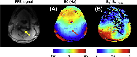
Rapid changes in B 0 arising from tissue interfaces with different magnetic susceptibility (e.g., tissue and air) can significantly affect image quality in the spinal cord at ultra-high field. For certain acquisitions (e.g., echo planar imaging, EPI), these susceptibility effects can result in significant geometric distortions and transverse magnetization dephasing, or signal “drop-out,” that scale with field strength. For example, artifacts shown in Chapter 2.3 would be even more exacerbated at 7 T, as the amount of distortion is proportional to B 0 . For the spinal cord in particular, susceptibility-related artifacts can arise from a number of structures (susceptibility mismatch between the vertebral bodies and surrounding tissue/cerebrospinal fluid or between the bony structures and the disc space), and can be time varying (cardiac pulsation, respiration). Thus, the spinal cord experiences a combination of global, slowly spatially varying perturbations in B 0 , local variation along the extent of the cord, and a rapidly time-evolving component. An example of a typical axial 7 T B 0 map at the level of C3 is shown in Figure 2.4.1 (A) with a resolution-matched anatomical image showing the location of the spinal cord (arrow).
Given the small diameter of the cord, correcting the B 0 homogeneity within the axial plane may require sophisticated image-based shimming techniques with second- and/or third-order shimming. Thus, high field scanners need to be equipped with higher order shims that are not commonly implemented at lower fields in order to perform robust spinal cord imaging. For larger volumes along the rostral-caudal extent of the cord, more sophisticated approaches may be required (e.g., dynamic shimming for multislice acquisitions) due to the highly nonlinear nature of these perturbations. There are, however, available approaches that can mitigate many of the effects of the static field variations of the cord at lower field (see Chapter 2.2 ), though additional work is needed to evaluate their effectiveness at 7 T.
Perhaps a larger issue is that B 0 can dynamically change due to motion (e.g., CSF pulsation, swallowing, and breathing) such that changes in the thorax can affect the uniformity of B 0 elsewhere. For example, a previous 7 T study of the brain found up to a 5 Hz variation (peak-to-peak) in B 0 in the brain over the course of the respiratory cycle, and it was noted that this effect increased moving from anterior to posterior regions. Raj et al., noted similar effects that increased from the superior to inferior portions of the brain. Recently, it was shown that temporal variations in B 0 are even larger in the spinal cord due to its relative proximity to the throat and lungs. Fast, single-shot readouts (e.g., EPI) might be considered to reduce some of the effects of these temporal variations on image quality; however, these sequences typically suffer from a lower spatial resolution than is required for many applications. As a result, multishot sequences, which are much more sensitive to temporal variations in B 0 , are often required. As such, one must either (1) remove the dynamic variations prospectively and/or (2) estimate them and correct for their effects retrospectively prior to reconstruction. The former can be achieved via respiratory and/or cardiac gating or triggering or via breath-held sequences. The latter can be achieved via navigated sequences that measure and correct for the temporal variation in B 0 in the spinal cord. Prior to investigating each of these techniques, a thorough characterization of the spatiotemporal variation in B 0 in the spinal cord, along with identification of the sources and of these variations at 7 T, is needed.
2.4.1.2.3
Transmit Field Inhomogeneity
Sequences that rely on B 1 uniformity are further compromised when operating at 7 T, where the RF pulse wavelength becomes smaller than the dimensions of the body to be imaged. At 300 MHz (7 T) and above, standing wave and “near-field” phenomena give rise to large variations in the transmit RF field. Multichannel transmit systems, advanced RF pulse designs (e.g., SPOKES pulse, optimized adiabatic pulses, composite pulses ), and high-dielectric materials have all been employed to improve the transmit field homogeneity. While these approaches have not been demonstrated in practical applications, each is expected to improve the B 1 uniformity in the cord. Additional work is needed to evaluate which approaches are best suited for spinal cord imaging at higher field strengths. In instances where one is interested in only small axial volumes such as the spinal cord (∼1.5 cm in cross-sectional size), it should be noted that some of these approaches may be less valuable or necessary as the transmit field varies slowly relative to the diameter of the spinal cord. An example of this can be seen in Figure 2.4.1 (B). Note that while B 1 is relatively homogeneous across the diameter of the cord, it is approximately 50% of the nominal prescribed value based on assuming the field
Pros
- •
Increased SNR → can achieve higher spatial resolution or reduced scan time
- •
Increased spectral resolution → MRS, CEST
- •
Increased sensitivity to tissue susceptibility → fMRI, delineating tissue microstructure
- •
Prolonged T 1 → MT, CEST
Cons
- •
Increased power deposition → SAR
- •
B 1 inhomogeneity → inconsistent and/or reduced flip angles (variable contrast, reduced SNR)
- •
B 0 inhomogeneity → Susceptibility artifacts, signal voids in GRE imaging, periodic signal fluctuation
- •
Decreased T 2 and T 2 ∗ → spectral line broadening, lower SNR in DWI
- •
Decreased shimming effectiveness
- •
Cost/Site requirements
2.4.2
Anatomical MRI
As has been pointed out in earlier chapters, the spinal cord is a somatotopically organized structure. Therefore, the higher-resolution imaging afforded at 7 T provides the opportunity to better assess the precise locations of lesions in the cord and relate these to specific neurological dysfunction. Histopathologically, studies have shown spinal cord GM may contain lesions that are related to neurological dysfunction, and at higher resolutions it may be possible to visualize such lesions. Also, it may be possible to assess the health of the nerve roots, which convey information to and from the spinal cord. Damage to the nerve roots can mimic the deleterious neurological effects arising from spinal cord lesions. In conditions like spinal cord trauma, degenerative disc disease, or bony malformations, the nerve roots may be involved to a greater degree than the spinal cord itself. Finally, segmentation of the spinal cord may be related to the clinical presentation in multiple sclerosis. In previous studies, the focus has been on the C2-C3 junction and the cross-sectional area (CSA) is measured. Even with this coarse measure, the relationship between atrophy and neurological dysfunction may be appreciated. Even at 3 T, segmentation of GM and WM has shown promise and at 7 T the reliability of atrophy measurements may be significantly increased.
Generally speaking, a clinical spinal cord imaging study at lower field strength incorporates T 1 -weighted, T 2 -weighted, short-tau inversion recovery (STIR), and fluid attenuated inversion recovery (FLAIR) sequences, though other methods may also be used and tailored to the pathology of interest. Currently, there are a limited number of reports on spinal cord anatomical imaging at 7 T. In Sigmund et al., the authors demonstrated the impact of the higher SNR at 7 T over lower field strength, which they used to obtain higher spatial resolution. Specifically, they focused their attention on T 2 ∗ -weighted imaging with short echo times. From their presentation, subtle structures are well visualized within the cord.
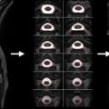
Other examples of 7 T anatomical MRI are given in Figure 2.4.2 , which shows that a nominal resolution of 0.3 mm in-plane can be readily achieved ( Figure 2.4.2 (A) ) using a conventional gradient echo sequence (all scanning details given at the end of the chapter). Note the greater detail seen of the gray matter in the lateral and dorsal horns. No longer is the butterfly-shaped gray matter simply a thin H-shaped structure in the body of the cord, but at this resolution, fine details of the lateral and ventro-lateral gray matter horns can be appreciated. In Figure 2.4.2 (F–G) a 1D phase navigator has been applied to each of five echoes and the first three echoes have been averaged to increase the contrast from the CSF, GM, and WM. In addition to the improved contrast within the cord, the spinal cord nerve roots can be visualized within the surrounding CSF using this technique.
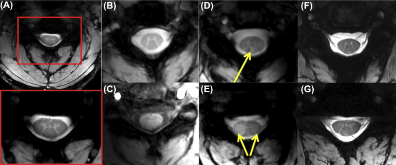
The increased SNR at high field can also be used to reduce acquisition times with resolutions comparable to conventional anatomical imaging at lower field strength. In Figure 2.4.2 (B–C), axial T 2 ∗ – and T 1 -weighted gradient echo acquisitions are shown at resolutions typical of 3 T MRI in the spinal cord (0.8 × 0.8 × 4 mm 3 ) and obtained in less than 8 min. In concordance with the fact that T 1 values for WM and GM are similar at lower field strengths, T 1 -weighted imaging of the spinal cord at 7 T shows little contrast between WM and GM ( Figure 2.4.2 (C)), especially when compared with the T 2 ∗ -weighted acquisition ( Figure 2.4.2 (B)). Similar T 2 ∗ -weighted images of the cervical spinal cord in a patient with multiple sclerosis are given in Figure 2.4.2 (D–E). Note the dorsal column lesion in panel D (arrow), and the bilateral tissue signal aberrations in the lateral columns in panel E (arrow).
To date, there have been no publications regarding spinal cord FLAIR or STIR at 7 T. Performing FLAIR imaging at 7 T is problematic due to the requirement of a uniform inversion RF pulse over the entire structure of interest, which for the brain is challenging, yet possible with tailored inversion and refocusing pulses, and alternative readout parameters. Recently, Zwanenburg and Visser proposed a high resolution 3D FLAIR for the brain. They showed that a T 2 preparation prior to inversion aided in enhancing the contrast between tissue types while minimizing T 1 contrast. The T 2 preparation consisted of a 90° pulse followed by a pulse train of adiabatic 180° pulses and a final 90° flip-back pulse. While not currently in use, this type of acquisition paradigm may prove to be equally beneficial for imaging inflammation in the spinal cord, and a similar preparation phase could easily be adopted for both FLAIR and STIR imaging.
Some preliminary reports demonstrated the benefits of 7 T for characterizing the pathological spinal cord in ALS and spinal cord injury. In the latter study, the high spatial resolution (300 micron in-plane) enabled the clear delineation of signal abnormality likely due to Wallerian degeneration of ascending dorsal column.
2.4.3
Quantitative MRI
2.4.3.1
Relaxometry
Relationships between relaxation parameters and microanatomical features such as myelination and iron content have previously been investigated with the goal of developing quantitative imaging biomarkers of disease. Unfortunately, while relaxation parameters are sensitive to overall tissue composition, they are not necessarily specific to a given microanatomical feature. There are, however, exceptions to this general rule. For example, Whittall and Mackay have shown that multicomponent characterization of white matter T 2 allows for the separation of the bulk signal into two components: (1) a short- T 2 from water residing between myelin bilayers and (2) a long- T 2 from water residing within and between axons. More recently, a relationship between the size of the short- T 2 and myelin content in the spinal cord has been shown, indicating that more specific information about myelination may be available via multicomponent relaxation measurements. It should be noted, however, that such measurements at 7 T are difficult because these sequences invoke high SAR and rely on the use of multiple refocusing pulses that are nonuniform at higher field.
In addition to providing information on tissue composition, NMR relaxation measurements at ultra-high field are essential for sequence optimization (e.g., optimization of white matter/gray matter contrast in T 1 -weighted scans). It is well known that T 1 increases while T 2 and T 2 ∗ decrease with increasing magnetic field strength. Thus, sequences that are optimized for spinal cord imaging at clinical field strengths yield suboptimal results at ultra-high field.
2.4.3.1.1
Spin–Spin Relaxation ( T 2 )
Spin echo sequences are most commonly used to measure T 2 . The spin echo signal S (TE) is given by:
S ( TE ) = S 0 e − TE T 2 + υ ,
υ
reflects noise, and TE is the echo time. In the ideal case, estimates of T 2 and S 0 can be obtained via nonlinear regression of images at different TE values to Eqn (2.4.1) ; however, variations in B 0 and B 1 can affect these estimates.
The spin echo signal is maximized when the refocusing pulse is a uniform 180° over the entire structure of interest; therefore, spin echo sequences are exquisitely sensitive to B 1 homogeneity. If one spin echo is acquired per TR, variations in the effective flip angle simply result in a reduction in the observed signal amplitude. For T 2 measurements, this reduction factor can then be folded into S 0 (Eqn (2.4.1) ), and the estimate of T 2 remains accurate. Often, however, multiple spin echoes are acquired per TR to more efficiently sample the T 2 decay curve. For multiple echo sequences, variations of this effective flip angle can result in signal contributions from non-spin echo pathways (e.g., stimulated echoes that evolve according to T 1 ) that cannot be accounted for by this simple model. In such cases, contributions from non-spin echo pathways must be minimized. At lower field strengths, composite (e.g., 90 x 180 y 90 x ) pulses are often used in concert with crusher gradients to minimize these non-spin-echo signal contributions. At 7 T, more robust pulses will likely need to be developed to account for B 1 inhomogeneity, especially when imaging over the rostral-caudal volume of the spinal cord in which we would expect a simultaneous variation in B 0 . It should be noted that such pulse designs often require high amplitude pulses; therefore, considerations of SAR are required when developing robust refocusing pulses for high field applications. In summary, T 2 estimation at high field is challenging, but there remain several options that warrant investigation.
2.4.3.1.2
Effective Spin–Spin Relaxation ( T 2 ∗ )
Spoiled gradient echo sequences, both single and multi-echo, are most commonly used to quantify T 2 ∗ . In this case, the observed signal equation can be expressed as:
S ( TE ) = S 0 e − TE T 2 ∗ + υ .
Again, in the ideal case, one can estimate T 2 ∗ via nonlinear regression of gradient echo images at different TE values to Eqn (2.4.2) . In reality, the signal from gradient echo sequences is also sensitive to spatial variations in B 0 , or background field gradients. Thus, in the presence of a background field gradient, the signal equation must be altered to include an additional term <SPAN role=presentation tabIndex=0 id=MathJax-Element-4-Frame class=MathJax style="POSITION: relative" data-mathml='fΔϕ’>fΔϕfΔϕ
f Δ ϕ
that accounts for background-gradient-induced signal loss:
S ( TE ) = S 0 e − TE T 2 ∗ f Δ ϕ ( TE ) + υ .
Related posts:


Stay updated, free articles. Join our Telegram channel

Full access? Get Clinical Tree


