Metrics
Explanation
Instruments
Sensors
References
Time (s)
Time taken to complete the procedure
Flexible/rigid
0
Path length (m)
Total distance travelled by the instrument
Flexible/rigid
1 (PS)/EC
Flex (m)
Difference in path length of distal and proximalend of instrument
Flexible
2 (PS)/EC
Velocity (m/s)
Rate of change of position
Flexible/rigid
1 (PS)/EC
Acceleration (m/s2)
Rate of change of velocity
Flexible/rigid
1(PS)/EC
Jerk (m/s3)
Rate of change of acceleration
Flexible/rigid
1 (PS)/EC
Tip angulation (rad)
Angulation of distal end of the instrument
Flexible
2 (POS)/EC
Angular velocity (rad/s)
Rate of change of angulation of the distal end
Flexible
2 (POS)/EC
Rotation (rad)
Total operational turn for the sensor
Flexible/rigid
1 (POS)/EC
Curvature (mm−1)
Derivative of the tangent vector (to the instrument shape) with respect to path length
Flexible
2 (POS)
Global isotropy index
Ratio of minimum to maximum singular value of the Jacobian matrix of a robot model for instrument throughout the entire duration – global value
Flexible/rigid
>2 (POS)/EC
[15]
Condition number
Ratio of the maximum to minimum singular value of the Jacobian matrix of a robot model for instrument at any instant
Flexible/rigid
>2 (POS)/EC
[15]
Depth perception (m)
Distance travelled by instrument along its axis
Flexible/rigid
1 (PS)/EC
Number of movements
Number of hand movements calculated from position data
Flexible/rigid
I (PS)/EC
Force (N)
Force applied on the instrument
Flexible/rigid
1 (FS)
Vosburgh et al. [16] describe the evaluation of the benefits of an augmented reality system to guide an endoscopic ultrasound (EUS) procedure. The hypothesis is that the use of the augmented reality display improves operator performance and enables smooth and accurate motion of the probe. Operator performance was measured with and without the display. Kinematic parameters which characterize the smoothness and efficiency of the motion (such as velocity, acceleration, angular velocity) were computed from the position and orientation of sensors attached to the echoendoscope. It was determined by comparing such metrics that the augmented reality display improved the performance of a user. The Imperial College Surgical Assessment Device (ICSAD) is a commercially available electromagnetic tracking system (Isotrak II, Polhemus, United States) that tracks the surgeon’s hands during a procedure. Studies on this simulator have shown that experienced and skilled laparoscopic surgeons are more economical in terms of the number of movements and more accurate in terms of target localization and therefore use much shorter paths [36, 37]. Similarly, the advanced Dundee endoscopic psychomotor trainer (ADEPT) [18] was developed for selection of trainees for endoscopic surgery, based on their innate ability to perform relevant tasks. Agarwal et al. [19] developed a method to assess surgical skill using video and motion analysis for laparoscopic procedures. They have shown significant differences between the novice and experienced groups of surgeons in terms of time taken, total path length, and number of movements. Cristancho et al. [33] have shown that a Principal Component Analysis performed on a six-vector component consisting of the lateral, axial, and vertical tool-tip velocities for two laparoscopic subtasks resulted in two dominant components which accounted for approximately 90 % of the variance across all subjects and tasks. In addition, it was also shown that novices have significantly higher velocities and frequency components in the motion trajectories compared to experts. This was also seen in the work by Megali et al. [34], wherein the Short-Time Fourier Transform showed higher frequency components for novices. This is expected since the laparoscopic tool, being rigid, follows the motion of the user. A novice has a tendency of manipulating the tool with greater velocity and jerks, resulting in higher frequency components, compared to the smooth, fluid motion of an expert. McBeth et al. [42] demonstrated, using a kinematic and video analysis of the motion of a laparoscope, that a single surgeon performing many cholecystectomies had consistent performance, which suggests that kinematic-based metrics are robust in this realistic setting.
Often, the difficulty is finding a kinematic metric which clearly differentiates surgical expertise. Robust and easy to compute metrics were developed for surgical procedures and combined to comprise the C-PASS performance assessment method [43] to assess surgical expertise. Neary et al. [20] showed that expert surgeons performed significantly better than the novice laparoscopic colorectal surgeons in terms of instrument path length, smoothness, and time taken to complete the procedure. This agrees with the work of others [19, 33, 34]. Zheng et al. [44] studied the work of teams while performing laparoscopic surgery and developed a simulator to train the team. During this process, they developed a video-based analysis of the laparoscopic tools with the hypothesis that surgical teams with longer teamwork experience resulted in more “anticipatory” motions of the laparoscopes [45]. Jayaraman et al. [46] developed a novel hands-free, head-controlled, and multimonitor pointer to improve instruction efficiency during advanced laparoscopic surgery. The primary outcome of time required to locate 10 points was shorter with the pointer than with verbal guidance alone.
The methods and metrics developed for laparoscopy require enhancement to accommodate flexible instrument manipulation. Flexible endoscopy, more specifically colonoscopy, has not received the same amount of attention as that received by laparoscopy [47, 48]. Ferlitsch et al. [21] quantified the expertise of the clinicians on a GI Mentor (Simbionix, Cleveland, OH) simulator using tactile and position feedback. It was shown that the group which underwent training was subsequently better at endoscopy. A similar study on the GI Mentor II [49] on 20 residents randomly split into two groups of training and no-training showed a significant performance improvement for the training group while inserting the endoscope into the esophagus for examination of the duodenal bulb and the fornix. Another study on the GI Mentor simulator showed that fellows trained using the simulator showed higher competency in the first 100 cases compared to their no-training counterparts [50]. For colonoscopy, the procedure time, specifically the withdrawal time during which the inspection takes place, is an important surrogate marker for overall procedure quality during colonoscopy [51]. A novel wireless Colonoscopy Force Monitor (CFM) [38] has been developed to measure the force applied at the proximal end of colonoscope as it is inserted. The results show that the amount of force exerted at the proximal end can be used to distinguish the expertise of the clinician. However, the introduction of the CFM could lead to user interface problems and difficulty in manipulating the colonoscope.
Case Study 1
To Compare a Navigation Display Consisting of Endoscopic Ultrasound (EUS) and CT to Conventional EUS for Targeting Fine–Needle Aspiration of Pancreatic Tumors.
In this case study [16], we show how kinematics based on deterministic metrics can be utilized in evaluating the efficacy of a navigation software for identifying key abdominal structures. The image registered gastroscopic US (IRGUS) system is a real-time guidance system that uses 2 synthetic displays driven by the position of the US probe to provide positioning, navigation, and orientation to the clinician.
Material and Methods
The IRGUS system provides the clinician with two contemporaneous real-time displays that display the probe within a 3D patient-specific model. Two synthetic images were then created, as shown in Fig. 8.1: (1) 3D models of reference anatomy with the endoscope tip and ultrasound image plane registered to the model and (2) a single oblique planar slice that matches the plane sampled by the US transducer. The synthetic images have no perceptible lag when the probe is moved. To evaluate the utility of the IRGUS system, a sample of expert (n = 5) and novice (n = 5) users were asked to identify 8 key anatomic landmarks in 5 min by using both traditional EUS systems and the IRGUS system in live anesthetized pigs. Novices were gastroenterologists with significant experience in endoscopy but less than 6 months of EUS training; experts were senior endosonographers from the US and European academic institutions but with only limited experience in the porcine model. All participants first used standard EUS, and in a later session the same day, but not back to back, they used the IRGUS system. All examinations were performed in the same study animal. Participants were asked to identify 8 structures. An instructor asked study participants to identify each structure as they progressed through the examination, and each answer that was provided was evaluated by a scoring panel. The data are reported as the ratios: (sum of answers provided) to (sum of questions asked) and (sum of correct answers) to (sum of answers provided). In other words, these numbers represent the probability of a person using EUS or IRGUS to provide an answer (label a target) and the probability of this answer being the correct one (accuracy). The position and the orientation of the probe were measured continuously during the procedures. These data were then used to calculate a set of kinematic metrics to correlate with performance. These included smoothness of motion, path length, and instrument rotation.
Fig. 8.1
IRGUS system display. The pancreas (yellow) and left kidney are shown in the ultrasound plane (top left) and the cropped preoperative CT (top right). Bottom, 3D view of the patient anatomy with the EUS probe shown in blue and black and the ultrasound plane shown in green, close to the pancreatic tumor
Results and Discussion
In the 5-min timed trial, both novice and expert endosonographers were able to locate and identify roughly twice as many abdominal organs and landmarks when using IRGUS compared with conventional EUS. Novice structure identification improved uniformly, except in respect to the right kidney, for which there was no improvement, with 40 % of users correctly identifying the structure with both EUS and IRGUS. The most significant improvements for experts were in identifying the porcine pancreatic tail and the right lobe of the liver; however, there was substantial improvement in identification of all structures. With IRGUS, users were also more accurate in structure identification (Table 8.2). For novices, the mean score with EUS was 0.29 versus 0.51 with IRGUS (P = .02). For experts, the score was 0.71 versus 0.80 (EUS vs IRGUS, respectively; P = .03)
Table 8.2
EUS versus IRGUS of the percentage of structures that were identified by study participants
% Total | % Correct | |
|---|---|---|
Novice | ||
EUS | 46 | 64 |
IRGUS | 58 | 100 |
Experts | ||
EUS | 71 | 86 |
IRGUS | 91 | 100 |
In the EUS timed trial, a novice had a 46 % probability to label a requested target by using EUS, with a 64 % accuracy (64 times of 100, this answer is correct). In contrast when using IRGUS, the probability of labeling a target increased to 58 %, with 100 % accuracy (P = .01). The experts had a 71 % probability to label a requested target when using EUS, with 86 % accuracy. In contrast when using IRGUS, this probability increased to 91 %, with 100 % accuracy (P = .004). The difference between novices using IRGUS and experts using simple EUS was not statistically significant (P = .32), which indicates that IRGUS closes the performance gap between experts and novices. The kinematic evaluation for the IRGUS versus EUS systems showed overall improvement in efficiency of examination with IRGUS, with score improvements that ranged from 17 to 27 % (Fig. 8.2). All users reported that the displays of (1) global position and orientation and (2) CT-US slice comparison were naturally intuitive and greatly facilitated target identification and probe positioning. All IRGUS users also reported that the tracker system gave additional confidence in image interpretation. In this case study, IRGUS operators identified anatomic features and navigated in the body more confidently than with conventional EUS. Compared with EUS, IRGUS provided more efficient scope movement and enabled users to more easily identify and distinguish between structures, such as the right and left lobes of the liver. The performance of both novices and experts improved with IRGUS in terms of structure identification and kinematics.
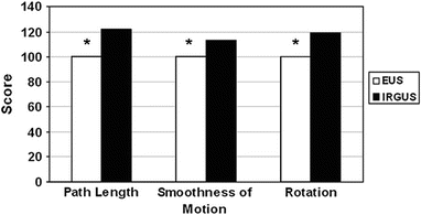
Fig. 8.2
Comparative scores for various kinematic factors for EUS and IRGUS, showing that the kinematics of IRGUS users was favorable for the parameters measured. The asterisk denotes that the difference between the 2 groups is statistically significant at the level of P < .05
Case Study 2
To Evaluate Expertise of Colonoscopists Using a Robotic-Based Dexterity Metric, the Global Isotropy Index [ 15]
We consider here the development of a composite metric to better differentiate classes of operators, that is, to separate “novice” from “expert” classes. This will enable training to proceed with more confidence. In this case study, we have utilized the Global Isotropy Index (GII) to quantify the expertise of the operator.
Material and Methods
The experimental setup consisted of a pediatric colonoscope equipped with four electromagnetic 6-DOF position sensors, as shown in Fig. 8.3. Male and female patients scheduled to undergo screening colonoscopy were enrolled in the research study. The effective sensor workspace covered the entire abdomen. Data are captured in real time starting from the insertion of the colonoscope into the anus and ending with the completion of the colonoscopy. Only the insertion phase of the procedure is analyzed since it is more difficult to insert a hyperflexible tube into the colon than to retract it.
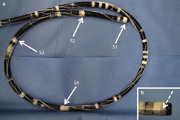
Fig. 8.3
(a) Colonoscope showing the position of sensors 1, 2, 3 and 4. (b) Magnified view of the colonoscope tip showing the sensor attachment
The colonoscope is modeled as a set infinitesimal rigid links along a backbone curve defined in terms of the Frenet-Serret frame. The curve is represented in the parametric form,  , where σ is the parameter which represents the curve length and t is the time. The Frenet-Serret frame is defined at each point p(σ,t) along the backbone curve and consists of the tangent
  , normal
  , and binormal
  vector at point p(σ,t), as shown in Fig. 8.4. Each segment of the colonoscope can be considered to consist of two rotational joints and a prismatic joint. The joint angle vector can be written as
 ![$$ \text{ }\overline{\theta }=\left[\begin{array}{ccc}0& \varsigma & \tau \end{array}\right]$$](/wp-content/uploads/2016/08/A176364_1_En_8_Chapter_IEq00085.gif) , and the translational vector can be written as
, and the translational vector can be written as ![$$ \overline{d}={\left[\begin{array}{ccc}{l}_{x}& 0& 0\end{array}\right]}^{t}$$](/wp-content/uploads/2016/08/A176364_1_En_8_Chapter_IEq00086.gif) , where l x is the extension of the length of the colonoscope, ς is the curvature, and τ is the torsion.
, where l x is the extension of the length of the colonoscope, ς is the curvature, and τ is the torsion.
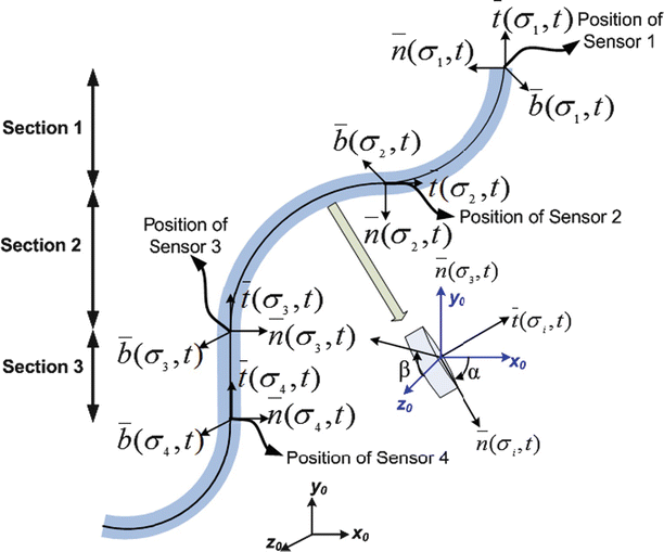
, where σ is the parameter which represents the curve length and t is the time. The Frenet-Serret frame is defined at each point p(σ,t) along the backbone curve and consists of the tangent , normal , and binormal vector at point p(σ,t), as shown in Fig. 8.4. Each segment of the colonoscope can be considered to consist of two rotational joints and a prismatic joint. The joint angle vector can be written as , and the translational vector can be written as , where l x is the extension of the length of the colonoscope, ς is the curvature, and τ is the torsion.Fig. 8.4
Model for colonoscope
At any point  along the curve
  , the local frame with respect to the base coordinates
  can be defined as
![$$ \begin{array}{cc}{}^{0}\Phi (\sigma ,t)=& \left[\begin{array}{ccc}\mathrm{cos}(\sigma \varsigma )\mathrm{cos}(\sigma \tau )& -\mathrm{sin}(\sigma \varsigma )& \mathrm{cos}(\sigma \varsigma )\mathrm{sin}(\sigma \tau )\\ \mathrm{sin}(\sigma \varsigma )\mathrm{cos}(\sigma \tau )& \mathrm{cos}(\sigma \varsigma )& \mathrm{sin}(\sigma \varsigma )\mathrm{sin}(\sigma \tau )\\ -\mathrm{sin}(\sigma \tau )& 0& \mathrm{cos}(\sigma \tau )\end{array}\right]\end{array}$$](/wp-content/uploads/2016/08/A176364_1_En_8_Chapter_Equ00081.gif)
along the curve , the local frame with respect to the base coordinates can be defined as(8.1)
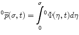
The position vector  of a point on the curve relative to the origin
  can be computed by integrating infinitesimal curve lengths along the tangent vector and is given by
The linear  and rotational velocity
  for a joint in the local Frenet-Serret frame with respect to the base frame can be derived as continuum extension for rigid link robots. Using the standard robotic terminology, the Jacobian operator can be defined as
![$$ \begin{array}{cc}J(\sigma ,t)=& \begin{array}{cc}{\displaystyle {\int }_{\text{}}{}{}0}^{{}{}\sigma}\left[\begin{array}{c}{}^{\sigma }\Phi (\nu ,t)\text{}[p(\nu ,t)-p(\sigma ,t)\times ]{}\Phi (\nu ,t)\\ 0\Phi (\nu ,t)\end{array}\right]& \overline{A}(.)d\nu \end{array}\end{array}$$](/wp-content/uploads/2016/08/A176364_1_En_8_Chapter_Equ00083.gif)
where
![$$ \overline{A}=\left[\begin{array}{c}1{}0{}0{}0{}0{}0\\ 0{}0{}0{}0{}0{}0{}1\\ 0{}0{}0{}0{}0{}1{}0\end{array}\right]{}{}{}\text{and}{}{}{}\text{{0.05em}}[a\times ]=\left[\begin{array}{ccc}0& -{a}_{z}& {a}_{y}\\ {a}_{z}& 0& -{a}_{x}\\ -{a}_{y}& {a}_{x}& 0\end{array}\right]$$](/wp-content/uploads/2016/08/A176364_1_En_8_Chapter_Equa.gif)
of a point on the curve relative to the origin can be computed by integrating infinitesimal curve lengths along the tangent vector and is given by(8.2)
and rotational velocity for a joint in the local Frenet-Serret frame with respect to the base frame can be derived as continuum extension for rigid link robots. Using the standard robotic terminology, the Jacobian operator can be defined as(8.3)
The colonoscope is considered to consist of three segments, defined by the four attached sensors placed along the colonoscope. For each segment of the scope, we assume that the consecutive sensors represent the base- and end-effector coordinates of the segment and solve the inverse kinematic problem to evaluate the configuration q = (σ, ς, τ) of the scope. We then solve the inverse kinematic problem to determine the configuration of the scope for a given set of base- and end-effector coordinates. The problem is formulated as a dynamical problem requiring only the computation of the forward kinematics, as determined by (8.2). The Jacobian matrix J(σ,t) relates the end-effector frame forces f to the corresponding joint torques τ, as given by the following equations

The Global Isotropy Index (GII) [52] was proposed to define the force isotropy throughout the workspace. The GII is used in this paper to define a global metric for evaluating the expertise of the clinician in actuating the distal end of the scope from the proximal end. The GII is defined as
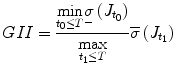 where T is the duration of the procedure, t 0 and t 1 are two instants during the procedure,
  , and
, and  are the minimum and maximum singular values of the Jacobian. GII is a global variable which determines the isotropy or the uniformity of the force transmitted to the distal end from the proximal end. Since the goal of colonoscopy is to uniformly transmit forces to the distal end of the scope, GII provides a metric for the expertise in manipulating the distal end of the scope while minimizing the amount of flexing caused due to excessive curvature in the scope. It is a stringent metric which quantifies the worst case performance of the user. Often this is the point at which the expert proctor takes over the procedure from the novice.
(8.4)
, and are the minimum and maximum singular values of the Jacobian. GII is a global variable which determines the isotropy or the uniformity of the force transmitted to the distal end from the proximal end. Since the goal of colonoscopy is to uniformly transmit forces to the distal end of the scope, GII provides a metric for the expertise in manipulating the distal end of the scope while minimizing the amount of flexing caused due to excessive curvature in the scope. It is a stringent metric which quantifies the worst case performance of the user. Often this is the point at which the expert proctor takes over the procedure from the novice.Results and Discussion
Five experts and four novice GI endoscopists (second- and third-year resident physicians) were recruited for this study. Thirteen screening colonoscopies were performed by the group (8 by experts and 5 by novices). All the colonoscopies were successful, leading to intubation of the terminal ileum. The positions of the 4 sensors were recorded, and the insertion and retraction phases of the procedure were tagged. Figure 8.5 shows the trajectory of sensor 2 for a novice and expert trial. Several kinematic parameters were computed from the position and orientation data and are shown in Table 8.3. The average time taken to complete insertion of the colonoscope from the anus to terminal ileum for the expert group was 564 s while the novice group took an average of 1,365 s to complete the same task. The path length, defined as the total distance travelled by the sensor, was also computed for the four sensors. In addition, a spline was interpolated between the position readings of the four sensors while maintaining the constraints of the length of the colonoscope between the sensors. The curvature of the three sections of the colonoscope was computed at each time point, based on which the mean curvature is calculated. The curvature provides insight into the amount of flexing in the scope as it is advances in the colon. At every time point, the position readings of the four sensors are also input to the continuum robot module, which calculates the configuration (σ, ς, τ) of the three segments of the colonoscope using the four sensor readings. Based on the configuration of the scope, the Jacobian of the scope and the minimum and maximum singular values are evaluated at each time point. A search algorithm obtains the minimum and maximum singular values of the Jacobian for the duration of the experiment, based on which the GII is calculated. The experimental results are shown in Table 8.3.
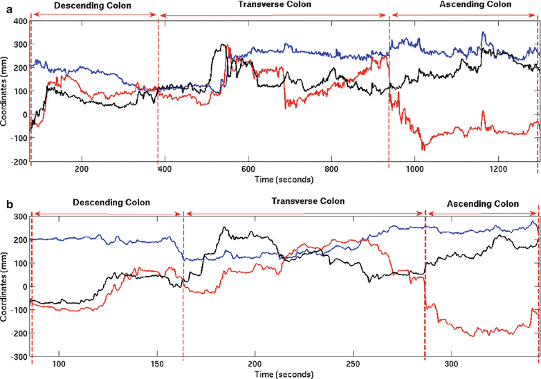
Fig. 8.5
(a) Trajectory of sensor 2 for novice trial, (b) trajectory of sensor 2 for expert trial
Table 8.3
Metrics for evaluating clinician’s performance
Time (s) | Pathlen (m) | Av.Vel (m/s) | Av.Acc (m/s2) | Av.Ang.Y (segrees) | Av.Ang.Z (degrees) | Av.Roll (rev.) | Av.Curv (mm−1) | Av.Cond | GII (×10−3) | |
|---|---|---|---|---|---|---|---|---|---|---|
Novice | 1,365 | 32.3
Related posts:Stay updated, free articles. Join our Telegram channel
Full access? Get Clinical Tree
 Get Clinical Tree app for offline access

|