Abstract
Magnetic nanoparticles (MNPs) have gained significant attention in biomedical engineering and imaging applications due to their unique magnetic and mechanical properties. With their high magnetization and small size, MNPs serve as excitation sources for magnetically heating to destroy tumors (magnetic hyperthermia) and magnetically controlled drug carriers in magnetic drug targeting. However, effectively visualizing the distribution of MNPs during research or potential clinical use with low-cost modalities remains a critical challenge. Although magnetic resonance imaging provides pre- and post-procedural imaging, it is considered to be high cost, and real-time imaging during clinical procedures is limited. In contrast, ultrasound-based imaging methods offer the advantage of providing the potential for immediate feedback during clinical use and are considered to be a low-cost modality. Ultrasound-based imaging techniques, including magnetomotive ultrasound, magnetoacoustic tomography, and thermoacoustic imaging, emerged as promising approaches for imaging the distribution of MNPs. These techniques offer the potential for real-time imaging, facilitating precise therapy monitoring. By exploring the strengths and limitations of various ultrasound-based imaging techniques for MNPs, this review seeks to provide comprehensive insights that can guide researchers in selecting suitable ultrasound-based modalities and inspire further advancements in this exciting field.
Introduction
Magnetic nanoparticles (MNP) have found widespread applications in diverse research and clinical domains, including magnetic resonance imaging (MRI) [ ], magnetic particle imaging (MPI) [ ], oncology [ ] and regenerative medicine [ ]. Among these applications, MNPs in oncology holds great promise in the magnetically enhanced treatment of cancer, such as magnetic drug targeting (MDT) [ ] and magnetic hyperthermia (MH) [ ]. These techniques offer the potential for minimizing the side effects of cancer treatment while maximizing treatment efficacy. Beyond this, MNPs can also be used in ultrasound molecular imaging [ ]. Ultrasound molecular imaging leverages the unique properties of MNPs to enable targeted visualization of specific molecular markers or biological processes at the cellular level.
MDT involves coating the surface of MNPs with a suitable layer serving for both biocompatibility and colloidal stability. Afterward, they are loaded with chemotherapeutic agents, which are then injected (intra-tumoral, intra-arterial, intra-cavitary or intravenous). By applying an external static magnetic field, MNPs can be accumulated in specific targets within the body, including cancerous tissue. This external field further enhances the tumor’s natural permeability and retention effect [ ], leading to increased accumulation of the chemotherapeutic agents in the tumor region and enabling local drug release over time. Animal studies [ ] have demonstrated the efficacy of this approach, with up to 35 times higher drug concentrations achieved 24 h after application to the tumor area compared with systemic administration. Additionally, approximately 30% of cases exhibited complete tumor remission with minimal side effects.
In contrast, MH uses MNPs solely for localized heating of tumor cells, resulting in their destruction. The application is also the same as in MDT (intra-tumoral, intra-arterial, intra-cavitary or intravenous). The MH process involves applying an alternating field in the kilohertz range, where MNPs efficiently absorb magnetic energy and convert it into heat. MH typical induces a cytotoxic effect in tumor cells at temperatures at approximately 46°C [ ]. An advantage of MH is that it avoids the administration of potentially hazardous drugs. Both MDT and MH have specific requirements that must be met for the methods to be effective. In this context, understanding the distribution of MNPs within the tumor becomes crucial. Accurate imaging techniques are necessary to assess MNP distribution and to be able to optimize treatment strategies.
MDT and MH hold immense potential in the treatment of various diseases, including cancer, cardiovascular diseases [ ] and neurological disorders [ ]. However, several challenges must be addressed before their clinical application in the human body can be realized. Beyond the development of MNPs that can be produced in sufficient amounts that are reproducible and of pharmaceutical quality, these challenges include ensuring the safe and effective delivery of MNPs and optimizing the magnetic field parameters for optimal therapy. Both of these require precise and localized therapy monitoring and imaging of MNP distribution.
Although MNPs find utility as contrast agents in MRI and MPI, these technologies present limitations in imaging MNPs during the accumulation process of MDT or MH. MRI uses strong static and alternating magnetic fields to generate detailed images of internal body structures. When used in MRI, MNPs enhance imaging contrast and sensitivity by appearing as dark spots due to their magnetic properties, which cause signal extinction [ ]. For larger concentrations of MNPs, the MRI signal can disappear entirely, meaning that the signal does not scale directly with iron content [ ]. However, the application of MRI in MDT encounters constraints. The strong static magnetic field used to accumulate MNPs interferes with MRI signal processing, and the size of the magnet used in MDT is generally too large to fit into standard MRI tubes.
Similarly, MPI relies on the magnetic properties of MNPs, where they become magnetized in the presence of an external magnetic field and emit a detectable signal for reconstruction [ ]. Despite offering high-resolution images and the potential for real-time imaging, it faces similar challenges as MRI in MNP imaging. Moreover, both MRI and MPI are considered high-cost modalities and are expensive to operate. Nevertheless, MRI and MPI remain promising imaging modalities for pre-therapy imaging to plan the treatment or, in case of MPI, for therapy monitoring after the accumulation process [ ].
Other methods for imaging MNPs, such as positron emission tomography [ ], single photon emission computed tomography [ ], alternating current biosusceptometry [ ] and magnetic relaxometry [ ] exist (see Table 1 for more methods). However, they encounter similar challenges as MRI or MPI when used with MDT and MH or are still in early research phases. In contrast, ultrasound-based methods provide a promising solution for imaging MNPs during MDT and MH therapy. Ultrasound is cost effective, offers high-resolution imaging, and enables real-time visualization, but classical ultrasound imaging cannot image these small MNPs. However, ultrasound-based modalities like magnetomotive ultrasound (MMUS) [ ], magnetoacoustic tomography (MAT) [ ] and photoacoustic imaging [ , ] have demonstrated their potential for imaging and quantifying MNPs distribution [ , ]. These ultrasound-based methods showcase the great potential of ultrasound in mapping the distribution of MNPs during therapy.
| Terminology | Selected Publications |
|---|---|
| Magnetic resonance imaging | [ , , ] |
| Magnetic particle imaging | [ , ] |
| Positron emission tomography | [ , ] |
| Single photon emission computed tomography | [ , ] |
| Magnetic relaxometry | [ , ] |
| Optical coherence tomography | [ , ] |
| Magnetomotive optical coherence tomography | [ , ] |
| Alternating current biosusceptometry | [ , ] |
| Permeability tomography | [ ] |
This review aims to provide an overview of ultrasound-based methods for imaging MNPs distribution. These methods are described, compared and discussed, offering a cohesive understanding of their capabilities. By highlighting the advantages and limitations of each technique, this review aims to shed light on the potential of ultrasound-based methods in MNPs imaging and stimulate further advancements in the field.
Accumulation and properties of MNPs
The properties of MNPs and the accumulation process in the biological environment significantly influence potential imaging methodologies. One of the most crucial factors for therapy and imaging is the MNP concentration (iron per volume: mg Fe/mL), which varies depending on the accumulation process. As mentioned in the introductory secton, the accumulation process during MDT and MH depends on the injection method (intra-tumoral, intra-arterial, intra-cavitary or intravenous), the applied magnetic field and the permeability and retention effect of the tumor. Determining the iron concentration achieved through these accumulation processes is challenging as this property is not well-documented in the literature, but some information is available.
Giustini et al. [ ] injected an MNP solution (5 mg Fe/mL) directly into the tumor region, with a relative distribution of 0.34 mL MNP solution per cm 3 tumor. Giustini et al. [ ] demonstrated a tumor uptake of up to 100%. This resulted in an MNP concentration inside the tumor of 1.7 mg Fe/mL. Huang and Hainfeld [ ] investigated intravenous MNP cancer hyperthermia in a mouse model. They reported an iron concentration of 1.9 mg Fe/mL inside the tumor using intravenous injection via a tail vein at 1.7 g Fe/kg body weight. Both experiments did not use a magnetic field for the accumulation process and were conducted on simple models.
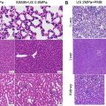
Tietze et al. [ , ] used rabbit models to demonstrate the advantages of intra-arterial injection with an external magnetic field over intravenous injection. They showed improved accumulation of MNPs in the tumor and reduced accumulation in the liver. The injected amount was 2 mL of lauric acid coated MNPs with mitoxantrone and an iron concentration of 4 mg Fe/mL. They reported an iron concentration of approximately 0.1 to 0.3 mg Fe per cm 3 tumor tissue. The lower amount of iron concentration compared with Giustini et al. [ ] and Huang and Hainfield [ ] can be explained due to the different approaches for injection and the larger animal. Giustini et al. [ ] used intra-tumoral injection, which should lead to the highest iron concentration of the discussed injection methods. Huang and Hainfeld [ ] used intravenous injection but with a less practicable setup than Tietze et al. [ , ]. One has to also keep in mind that the particles are not distributed homogeneously in the tumor tissue and the iron concentration can be higher in local regions.
High iron concentrations in MH studies have also been reported. For instance, Johannsen et al. [ ] conducted a clinical study on humans using an aqueous solution with an iron concentration of 120 mg Fe/mL, where 12.5 mL of this solution was injected directly into the prostate tumor. The total iron uptake was not specified due to the nature of the human trial, but their prior animal studies on rats showed an iron uptake ranging from 53% to 79% of the injected amount in the prostate with a lower iron concentration of 41.7 mg Fe/mL [ ]. In clinically relevant scenarios, an iron uptake of 0.25% to 1.00% of the total injected iron content is to be expected [ ].
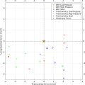
The upper and lower imaging thresholds for iron concentration vary significantly depending on the application; the used MNPs’ iron concentration can range from hundreds of qg Fe/mL to tens of mg Fe/mL. However, from the presented data, an imaging system should ideally be capable of detecting an iron concentration around 1 mg Fe/mL, with a target of 0.1 mg Fe/mL or less for enhanced imaging to accommodate various applications. Imaging methods that use higher iron concentrations should not necessarily be considered worse, but rather suitable for different specific applications.
Not only the concentration but also the properties of the MNPs are important. MNPs typically consist of an iron core (either single core or agglomeration) and a coating for biocompatibility and stability. The size of the MNPs impacts the accumulation process and possible concentration levels [ ]. Whereas the shape of the MNPs also influences their behavior [ ]. For MDT applications, drugs are often bound to these particles. The synthesis and coating methods significantly impact MNP properties. Common synthesis methods include co-precipitation [ ], a hydrothermal method [ ], thermal decomposition [ ] and a polyol method [ ], among others [ , ].
In this review, MNPs are simplified to an iron core with a core size in nm, and an outer shell or coating with a hydrodynamic size in nm (core size + shell thickness). The synthesis method will not be covered. Interested readers should refer to the cited literature for more detailed information. Relevant parameters for this contribution include the magnetic core size, the hydrodynamic size, the coating and the magnetic properties (susceptibility and magnetization). For a more detailed description of MNPs for biomedical purposes, refer to [ , ] and available sources.
Ultrasound-based methods
Ultrasound imaging has been used widely for decades to visualize internal structures in medical and material testing applications. Although it is primarily known for its use in imaging, ultrasound has also found applications in therapeutic ultrasound [ ], ultrasound hyperthermia [ ] and ultrasound non-destructive testing [ ]. Moreover, within the field of nanomedicine and nanostructures, ultrasound has been used for contactless nanomanipulation [ ], propelling nanorod motors [ , ], local drug release [ ] and much more.
In this section, we explore the various methods that have been developed and are being researched currently for imaging the distribution of MNPs in biomedical applications using ultrasound (refer to Table 2 ). Specifically, we explore techniques such as MMUS, MAT and thermoacoustic imaging. Each method will be explained in detail here and discussed in the following section. Furthermore, an outlook on future developments is provided.
| Terminology | Physical Property | Type of Nanoparticle |
|---|---|---|
| (Quantitative) Magnetomotive ultrasound | Magnetic permeability/magnetism | MNPs |
| Magnetomotive shear wave elastography | Magnetic permeability/shear strain | MNPs |
| Magnetoacoustic tomography with magnetic induction | Conductivity/electric | All |
| Magnetoacoustic tomography | Magnetic permeability/magnetism | MNPs |
| Magnetoacoustic concentration tomography with magnetic induction | Magnetic Permeability/Magnetic | MNPs |
| Photoacoustic imaging | Specific absorption rate | All |
| Magneto-thermoacoustic imaging | Hysteresis losses | MNPs |
| Ultrasound-guided magnetic hyperthermia | Hysteresis losses | MNPs |
For a broader understanding of ultrasound-based methods and nanoparticles, the interested reader may also refer to other review papers, such as Mallidi et al. [ ], which focuses on imaging various types of nanoparticles with ultrasound; Li et al. [ ], which highlights the applications of nanoparticles in ultrasound imaging and therapy; Shin et al. [ ], which explores imaging MNPs using various multi-modal imaging methods; Józefczak et al. [ ], which discusses ultrasound theranostics with magnetic mediators; Hosu et al. [ ], which focuses on MNPs in cancer detection, screening and treatment; and Nabeel Rashin and Hemalatha [ ], which explores the influence of magnetic and acoustic fields on magnetic nanofluids.
Magnetomotive imaging
During MH or MDT therapy, an external magnetic field is applied to accumulate the MNPs in the tumor region. This uses the magnetic properties of the MNPs for therapy purposes. Consequently, using ultrasound-based methods to image the distribution of MNPs by capitalizing on their property of being displaced by magnetic force would be a logical approach. When the particles move, they induce motion in the surrounding tissue, which can be mapped using ultrasound. This concept forms the basis of MMUS applications [ ].
MMUS encompasses various approaches, depending on the type of magnetic field used to induce displacement. In the typical MMUS approach, a sinusoidal excitation is used to induce displacement. Additional approaches include pulsed MMUS [ ], which uses pulsed magnetic fields, and coded MMUS [ , ], which uses either linear up-chirp or barker-coded excitation fields. Other MMUS methods, such as contrast-enhanced MMUS [ ] using microbubbles, quantitative MMUS [ ] aiming to quantify the distribution of MNPs and elastographic MMUS [ , ], which uses magnetomotive force to image the mechanical properties of surrounding tissue, are also used with MNPs.
For a comprehensive review specifically on MMUS, refer to Sjöstrand et al. [ ], and for a detailed review on magnetomotive imaging, consult Kubelick and Mehrmohammadi [ ]. Table 3 lists selected MMUS methods for an overview, and the subsequent subsections discuss the most significant ones.
| Terminology | Selected Publications |
|---|---|
| MMUS | [ , , ] |
| Coded MMUS | [ , ] |
| Pulsed MMUS | [ , , , ] |
| 3-D MMUS/pulsed MMUS | [ ] |
| Contrast-enhanced MMUS | [ , ] |
| Quantitative MMUS | [ , ] |
| Configuration Selected | Publications |
|---|---|
| Config (a) | [ , , – , , , , , , , , , ] |
| Config (b) | [ , , , ] |
| Config (c) | [ ] |
| Config (d) | [ , , ] |
| Config (e) | [ , , ] |
MMUS
The initial use of magnetomotive force to induce vibrations in a biological medium and subsequently investigate the induced motion with ultrasound can be traced back to a study conducted by McAleavey et al. [ ] in 2003. This study primarily assessed the feasibility of using this method for the detection of prostate brachytherapy seeds. Nevertheless, the formal introduction of MMUS as a distinct technique is attributed to the work of Oh et al. [ ] in 2006. In this research, the identification of tissue-based macrophages was achieved using MNPs and MMUS. In this method, a sinusoidal magnetic field displaces MNP within tissue or tissue-mimicking phantoms, causing the surrounding tissue to also move. First, this tissue movement was detected using an ultrasound system to measure induced Doppler shifts and image it with power Doppler and M-mode imaging. Later, MMUS was adapted to pulsed magnetic fields [ , , ] and its combination with photoacoustic [ ] and photothermal therapy [ ] was explored. The enhanced pulsed MMUS method used similar cross-correlation techniques as in ultrasound elastography, where the received radiofrequency data under different magnetic force deformations were analyzed. This approach was also used for detecting the intracellular accumulation of MNPs [ , ].
In later works, the phase information of the displacement was included in MMUS [ , ] to enhance its imaging robustness. It was stated in [ , ] that the MMUS algorithm, which uses sinusoidal time-varying magnetic fields and relies entirely on the magnitude of displacement, has problems distinguishing natural tissue displacement outside the MNP area from displacement due to magnetomotive force. Evertsson et al. [ ] introduced a high-frequency phase-sensitive MMUS approach that analyzes the phase of the displacement. This phase-sensitive approach has become widely implemented in MMUS and will be used in this section to explain the working principle of MMUS. The other implementations of MMUS follow a similar principle.
Evertsson et al. [ ] used an MMUS configuration, where the electromagnet and the ultrasound transducer were positioned on opposing sides (refer to Figure 1 a). The electromagnet emits a time-varying sinusoidal magnetic field B ( r , t ), that has the same frequency as the applied current of the electromagnet. As this magnetic field is applied to the imaging area, the magnetomotive force [ ]
F(r,t)mag−motive=∇(χSV2μ0|B(r,t)|2)=χSV2μ0∇(|B(r,t)|2)
where e z is a unit vector in z -direction. With this assumption about the magnetic field, the magnetic force from eqn (1) can be expressed as [ ]
F(z,t)mag−motive=χSV2μ0(1−cos(4πf0t))Bz(z)∂Bz(z)∂zez.

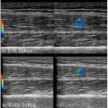
This equation provides interesting properties of the acting magnetomotive force, for example, the oscillation frequency of the MNPs is twice that of the applied magnetic field. Moreover, the larger the magnetic field, the magnetic field gradient, or the magnetic susceptibility of the MNPs, the larger the magnetomotive force. In classical MMUS approaches, the next step would involve measuring the magnitude of the induced displacement with ultrasound-based methods and identifying areas where the displacement frequency corresponds to twice the applied frequency. However, it has been demonstrated by Evertsson et al. [ ] that relying solely on displacement measurement does not exclude displacement in unwanted areas. Instead, they showed that the region containing MNPs oscillates not only twice the excitation frequency (2· f 0 ) but also with a phase shift of π compared with the surrounding tissue. Therefore, combining measurements of displacement and phase enhances the imaging of MNPs. Figure 2 from Evertsson et al. [ ] illustrates the results of this phase-sensitive MMUS approach ( Figure 2 d) compared with the classical approach ( Figure 2 b). Figure 2 a shows the total displacement and Figure 2 c the phase of the displacement.

To evaluate the effectiveness of the phase-sensitive MMUS approach [ ], a polyvinyl alcohol ultrasound phantom was prepared with three distinct regions ( Figure 2 ). Region I contained an MNP inclusion with an iron content of 0.6 mg/mL, and region III had an iron content of 0.45 mg/mL. Region II represented the normal polyvinyl alcohol ultrasound phantom without MNPs. The ultrasound transducer was placed above the phantom, coupled with ultrasound gel, and the excitation electromagnet was positioned below the phantom.
Figure 2 a displays the magnitude of the total induced displacement for all frequencies, where no clear distinction between the MNPs area and the normal ultrasound phantom area is visible. When examining only the magnitude of displacement corresponding to the excitation frequency ( Figure 2 b), region I becomes visible prominently. However, it is important to note that all other regions in the phantom also exhibit displacement at this frequency. This lack of specificity makes it impossible to distinguish between MNPs with lower iron content (region III) and artifacts. In Figure 2 c, the phase of displacement for all frequencies is shown. Areas with and without MNPs have a phase difference of π. Evertsson et al. [ ] attributed the phase difference of π to the rigid boundaries of the phantom mold. Due to these rigid boundaries, the displacement of MNPs must be counteracted with displacement in the opposite direction, resulting in the opposite phase. By using the areas with a phase difference of π from Figure 2 c as a mask for the displacement in Figure 2 b, a phase-sensitive MMUS image is generated ( Figure 2 d). This image primarily contains displacement information from regions I and III, where the MNPs inclusions are located. This highlights the improvement over the original MMUS method, which solely relied on the magnitude of the displacement. A finite element simulation of a comparable setup validated the effectiveness of the proposed MMUS method and provided valuable insights into MMUS movement patterns [ ]. The simulated MMUS image closely matched the measured displacement, with differences primarily in the noise pattern and the magnitude of the actual displacement.
It is interesting to note that the measured displacements of different publications differ in some magnitude. In the case of [ , ], the displacement magnitude is typically around 3 μm or lower. In contrast, earlier publications [ ] demonstrated displacements exceeding 100 μm, while subsequent works [ ] reported results in the tens of μm range. The discrepancy in displacement magnitude can be attributed to the different ultrasound phantoms used, the strength of the magnetic field applied, the MNP iron content, and the physical properties of the MNPs. For example, Levy et al. [ ] demonstrated the influence of the elastic parameters of the ultrasound phantom on MMUS displacement, where higher elastic moduli results in lower displacements. Additional approaches to enhance induced displacement include modifying the properties of the MNPs, such as using tailored MNPs [ ] or pre-magnetizing the MNPs [ ]. Furthermore, improvements can be achieved through coded excitation [ , ] to enhance the signal-to-noise ratio and robustness against interference [ ], as well as using more accurate displacement estimators [ , ]. It is worth mentioning that MMUS can also be combined with thermal strain imaging (see the Ultrasound-guided MH section) for imaging MH [ ].
Furthermore, it has been demonstrated that MMUS can be performed in near real-time, achieving a frame rate of 3.46 Hz [ ]. This represents a significant advancement compared with other MMUS implementations that require several seconds to minutes to compute the displacement map. There are additional approaches to further enhance the real-time capabilities of MMUS, such as using recursive estimators [ ] or implementing it online on an ultrasound system [ ].
The configuration used for MMUS, particularly the positioning of the magnet and ultrasound transducer, is crucial for its clinical applications. The original configuration ( Figure 1 a) with the magnet and ultrasound transducer on opposite sides of the imaging region presents practical challenges, such as large distances between them and limited space in operation rooms. Alternative configurations have been explored, as depicted in Figure 1 . These configurations have been extensively tested in ex vivo and in vivo experiments. The first MMUS imaging on living rats, focusing on tumor detection, was conducted by Mehrmohammadi et al. [ ]. In this study, a pulsed MMUS scheme was used to perform 3-D imaging of rat tumors, marking also the first instance of 3-D MMUS imaging. Furthermore, the development of a hybrid transducer (resembling the configuration shown in Figure 1 e) aimed at overcoming the spatial resolution limitations associated with alternating current biosusceptometry for MNP detection. This transducer has the capability to concurrently collect susceptometric and MMUS data [ ]. In vivo testing of this hybrid transducer demonstrated its potential for evaluating gastric function. Notably, the 3-D MMUS images produced by this transducer provided detailed anatomical information about the rat stomach [ ]. Ex vivo testing on rat lymph nodes was carried out [ , ], also in combination with other imaging modalities [ , ]. In vivo experiments were conducted on rats [ , ] and rabbits [ ]. Significantly, the study by Fink et al. [ ] marked the first instance of imaging the accumulation process of MNPs during MDT and using a setup in vivo where both the magnet and ultrasound transducer were positioned on the same side ( Figure 1 d), demonstrating the effectiveness of MMUS for MDT. However, the most advanced and nearly clinic-ready MMUS configuration involves a rectal probe with a revolving permanent magnet inside, surrounded by an ultrasound transducer array [ ] (patent pending [ ]). The rectal MMUS probe has been evaluated successfully on excised human tissue from a patient with rectal cancer, marking the first-ever human tissue trial of MMUS. A patient with advanced low rectal cancer was scheduled for rectal removal as part of tumor treatment. Before the surgery, 2 mL of MNPs solution (Magtrace, Endomag) was injected at three different sites: one directly into the tumor and two on either side of the tumor using an injection needle designed for hemorrhoids. After removal, the MMUS probe was able to image these three regions successfully. Furthermore, patents for MMUS were also granted or are pending [ , ].
Quantitative MMUS
Accurate quantification of the concentration of chemotherapeutic agents and MNPs at the tumor site is crucial for effective dose control and optimal treatment outcomes in MDT and MH. It is also important for molecular imaging to quantify where the particles accumulate. This information enables precise modulation of therapeutic interventions and ensures adequate heating in hyperthermia applications. The quantification of MNP distribution using MMUS was first explored in a simulation study [ ] in 2010. The study examined the design of magnetic coils to generate uniform magnetic fields for MMUS. They suggested that a uniform magnetic field would result in a displacement map proportional to the MNPs density if used in MMUS schemes.
Subsequently, research was conducted to quantify the effects of non-uniform magnetic fields and excitation parameters on magnetomotive displacement [ ]. Furthermore, Hossain et al. [ ] and Thapa et al. [ ] computed the normalized MNP density map by using the displacement excited by MNPs and the magnetic force in an inverse scheme. They successfully computed normalized MNPs density maps which are proportional to the MNP quantity, but only normalized and with halo-like artifacts.
In recent studies by Fink et al. [ , , ], a method was developed to quantify the absolute distribution of MNPs, rather than normalized maps. For this purpose, MMUS displacement maps were generated and measured using an ultrasound MNP phantom, in which displacements were induced by an external magnetic field. The displacement was measured using the frequency and phase sensitive approach from Evertsson et al. [ ], which results in u z ,meas ( x, y ).
Fink et al. [ ] assumes a linear mechanical model, as the tissue displacement is in the low micrometer range. Navier’s equation is used to formulate the differential equation
fV(Fmag−motive,d)+DTeDusim(x,y,z)=ρ∂2usim(x,y,z,t)∂t2,
D
the as differential operator, which links the induces stress to the corresponding volume force and e is the elasticity matrix in Voigt’s notation for isotropic materials. The elasticity matrix e includes two independent coefficients, the Lam parameters and describes the relationship between strain and stress in Hooke’s Law. A finite element simulation is used to solve eqn (4) , which is done in 3-D. Using the matrix e and the differential operator D
D
a 3-D simulation, which considers not only the axial displacement, but also the displacement due to shear stress and heterogeneous material parameters, computes u sim ( x, y , z). The magnetic gradient force F mag-motive is also simulated using a rotational symmetric finite element simulation. The simulated displacement u sim ( x, y, z ) = ( u x,sim ( x, y, z ), u y ,sim ( x, y, z ), u z,sim ( x, y, z )) T and the magnetic gradient force are a 3-D vector field (for more details about the simulation refer to Fink et al. [ ]). To compare it to the 2-D slice of the measured displacement u z ,meas ( x, y ), only a slice ( z = 0 is set to ultrasound imaging plane) of the axial ( z -direction) component of the simulated displacement is used, resulting in u z,sim ( x, y ). The MNP concentration is calculated using the maximum measured ( ˆumeas=max{uz,meas(x,y)}
u ^ meas = max { u z , meas ( x , y ) }
) and simulated ( ˆuz,sim=max{uz,sim(x,y)}
u ^ z , sim = max { u z , sim ( x , y ) }
) tissue displacement with
where the qualitative particle distribution
is normalized to its maximum
ζ = ζ 0 in eqn (5) is a random scalar value (has to be larger than zero), which exact value is not relevant. It is used to give the correct unit (particles per volume) to the distribution and to determine the optimal scaling of the quantitative distribution ζ opt . Equation (6) sets the qualitative MNP distribution in relation to the non-uniform magnetic field, while using the simulated displacement ˆuz,sim(x,y)
u ^ z , sim ( x , y )
sets the distribution in relation to the mechanical parameters ( ρ, e ).
An example of this result is depicted in Figure 3 . In this example, an MNPs concentration of 4 mg/mL, corresponding with 6.0·10 14 particles per mL, was used. As shown, the result matches the actual MNPs distribution. With this approach, only a single simulation of the displacement map needs to be performed and compared with the real data. Thus, the method’s speed is limited solely by the simulation time and does not encounter convergence issues. These findings demonstrate the potential of MMUS for quantitative imaging of MNPs.

For practical implementation, precise mapping of the elastic parameters of surrounding tissue remains an area of ongoing research. Fink et al. [ ] demonstrated that inaccuracies in assessing mechanical parameters for simulations can significantly impact the results negatively. This can hinder practical implementation, as accurately quantifying the elastic parameters of biological tissue is complex. The linear and elastic assumptions used in mechanical simulations can pose problems in real scenarios, such as near blood vessels. It is also important to note that Sjöstrand et al. [ ] evaluated finite element simulations for MMUS displacement estimation, highlighting the significance of mechanical coupling.
Furthermore, the method requires additional evaluation, as it assumes a linear relationship between measured and simulated displacements with a single scaling parameter for the entire distribution. Although the presented method claims to be an inversion technique, it lacks a defined inversion problem and a feedback loop. Additionally, the 3-D distribution of MNPs is assumed to be uniform outside the imaging plane or that no particles exist outside this plane. These assumptions are inaccurate and can affect the results. For a detailed discussion on the assumptions, refer to the conclusion of Fink et al. [ ]. The method proposed by Fink et al. [ ] shows promise and warrants further evaluation, but its practicality in real-world applications needs to be demonstrated.
Magnetomotive elastography
Obtaining information about the structure and function of tissue through the assessment of their mechanical parameters is an essential part of medical diagnosis and therapy. Ultrasound elastographic imaging offers a non-invasive means of measuring these mechanical parameters. Two commonly used methods within this field are ultrasound strain elastography [ , ] and ultrasound shear wave elastography (SWE) [ , ]. These techniques induce tissue displacement to assess the stiffness or elasticity of tissue, with Young’s modulus ( E ) and shear modulus ( G ) representing the resistance to deformation under compression (longitudinal stress) and shear stress (transversal stress) respectively. Both methods are clinically available, and some studies have reported using these techniques to image the distribution of MNPs [ ]. However, the existing literature is limited, and the experiments have primarily been restricted to simple phantom studies.
A promising approach involves using the magnetically induced displacement of MNPs to image mechanical parameters. This technique primarily aims to image tissue properties, but can also map the distribution of MNPs. Various methods exist within this approach. MMUS elastography, which is similar to traditional ultrasound elastography, has not yet been tested on MNPs [ ]. Another variant is MMUS-based resonant acoustic spectroscopy, which estimates Young’s modulus by comparing the simulated and measured mechanical spectral responses [ ]. However, MMUS-SWE emerges as the most promising approach, having undergone more extensive evaluation in the literature compared with other methods [ , ].
In standard ultrasound SWE, a radiation force impulse is emitted from an ultrasound transducer to mechanically displace the tissue and induce shear wave propagation. As the speed of the longitudinal wave is higher than the speed of the shear wave (e.g., c L = 1430…1579 m/s and c S = 2…6 m/s) [ ], the shear wave propagation can be tracked with ultrafast plane wave imaging and used to reconstruct a shear wave speed map. The shear wave speed can then be used to estimate the shear modulus and Young’s modulus.
In MMUS-SWE, MNPs and the magnetic gradient force ( eqn [1 ]) are used. Under the influence of this magnetic gradient force, induced by a time-limited harmonic [ , ] or a pulsed signal [ ], shear waves are excited and propagate. This propagation can be tracked using the pulse-echo method from Deng et al. [ ] or similar techniques to compute shear wave speed ( c S ), which is linked to shear modulus G
and, under the mechanical assumption of linear, isotropic, and homogeneous tissue behavior, also to Young’s modulus E,
with ρ as mass density. Lin et al. [ ] and Pi et al. [ ] evaluated this principle on phantom and in vitro experiments (see Figure 4 ), simulating or experimentally evaluating various scenarios.

The presented phantom experiment in Figure 4 used MNPs (10-30 nm, MACKLIN, China) in a gelatin mixture. A phantom with an MNPs inclusion and a non-MNPs inclusion ( α -Fe 2 O 3 , 10-30 nm) (Aladdin Scientific, Shanghai, China) was prepared. A magnetic field with a maximum magnetic flux density of 1.4 T and a pulse width of 380 μs was applied. The corresponding shear wave propagation of the phantom experiment is presented in Figure 4 , showing a B-mode image of the phantom with MNPs ( Figure 4 c) and the corresponding shear wave propagation ( Figure 4 d). The authors of [ ] also computed an MNP localization image using MMUS-SWE, where the maximum displacement of the first 20 frames and an 80% threshold is used to generate a binary mask, with the center representing the MNPs position. This localization image is presented in Figure 4 e.
The phantom experiments of [ ] and the in vitro experiments of [ ] demonstrated the potential to simultaneously image the MNPs distribution and the shear wave speed. Using the shear wave speed allows for estimations of the elastic parameters. However, in vivo experiments are needed to show the practicability of this method.
MNPs in magnetomotive imaging
Magnetomotive imaging represents one of the most advanced and mature techniques for imaging MNPs in ultrasound-based methods. MMUS, quantitative MMUS, and magnetomotive SWE are based on the magnetic displacement of MNPs as described by eqn (1 ). Beyond the magnetic gradient force, the viscous drag force and the elastic restoring force are also significant, influenced by the tissue environment and the mechanical coupling of MNPs to the tissue [ ]. Table 7 lists some MNPs used in magnetomotive imaging, categorized by the corresponding imaging method. The listed studies have used various MNPs with differing iron core materials, coatings, sizes and magnetic properties.
The experimental environment (phantom, ex vivo or in vivo ) significantly influences the resulting displacement, which must be considered when using magnetomotive imaging methods. It has been shown that MMUS can effectively image MNP distributions in phantoms with iron concentrations as low as 0.04 mg Fe/mL [ ]. However, this strongly depends on the experimental setup. For instance, Evertsson et al. [ ] reported that an iron concentration of 0.3 mg Fe/mL was insufficient for MMUS, attributing this to diamagnetic effects and mechanical parameters of the phantom which can result in a threshold phenomena. These variations highlight the importance of MNP type, elastic environment, and magnetic field used.
MMUS has been used successfully for imaging sentinel lymph nodes in rats with iron concentrations of 0.1, 0.2 and 0.3 mg Fe/mL after the subcutaneous injection of 0.1 mL MNP solution. Additionally, an experiment in human tissue was conducted using clinically available MNPs (Magtrace, Endomag) with a concentration of 26 mg/mL [ ].
QMMUS has been tested with MNP concentrations of 1 to 4 mg/mL, and MMUS-SWE with concentrations of 20 to 60 mg/mL, primarily in phantom studies. Among these methods, MMUS has shown the most promising results, while QMMUS and MMUS-SWE also demonstrated potential for diverse MNPs and practical iron concentrations. QMMUS and MMUS-SWE have to be tested and evaluated with lower iron concentration levels and in animal experiments to demonstrate their potential in clinically relevant scenarios.
Magnetoacoustic imaging
The term magnetoacoustic is used in different fields of engineering and physical studies (e.g., magnetoacoustic waves in plasma due to thermal pressure, magnetic pressure, and magnetic tension [ , ] or magnetoacoustics in biomedical imaging [ , , ]). To avoid confusion, the generation of acoustic signals due to magnetic heating is called magnetothermoacoustics and the generation of acoustic signals due to high-frequency mechanical movement is called magnetoacoustics. In this section, the focus is on exploring magnetoacoustic techniques in biomedical imaging that are based on eddy currents, Lorentz force and magnetomotive force without considering any heating processes or thermal change (see Table 5 ).
| Terminology | Input Signal | Physical Process | Output Signal | Selected Publications |
|---|---|---|---|---|
| MA Imaging | DC + AC MF | LF | US | [ , , ] |
| Hall-Effect Imaging | DC MF + US | LF | Voltage | [ , , ] |
| MA Tomography (MAT)/Detection (MAD) | DC + Pulsed (as) MF | Magnetic Force | US | MNPs: [ , , , , ] |
| MA with Magnetic Induction (MAT-MI) | DC + AC MF | Eddy Current and LF | US | [ , , , ]; MNPs: [ , , ] |
| MA Concentration Tomography with Magnetic Induction (MACT-MI) | DC + AC MF | Eddy Current, Magnetic Force and LF | US | MNPs: [ , , , ] |
| MA Tomography with Current Injection (MAT-CI) | DC MF + Electric Current | LF | US | [ , ] |
| MA-Electrical Tomography (MAET) | DC MF + FUS | LF | Voltage/Current | [ , ] |
| Hybrid MA Measurements (HMM) | DC MF + FUS | US + LF | US + Voltage | [ , ] |
The first time magnetoacoustics was used in a biomedical context to detect and image bioelectric currents was in 1988 by Towe and Islam [ ]. The process was then theoretically described by Roth et al. [ ] in 1994. In this paper, it was clearly illustrated, that the arising Lorentz force was used to image the bioelectric currents and that the excited displacement due to induced eddy currents was a problem. The historically next modality was introduced in 1997 by Wen et al. [ , ] and termed “Hall effect Imaging” in 1998, which illustrates how the Hall effect can be used to couple magnetic fields and ultrasound to generate conductivity maps.
Before 2005, significant progress in biomedical imaging using magnetoacoustics was limited. Although studies involving the coupling of electric or magnetic fields with ultrasound were conducted [ ] and a patent for magnetoacoustic imaging was granted [ ], it was not until Xu and He [ ] introduced MAT with magnetic induction (MAT-MI) that the field saw major advancements. The terminology of magnetoacoustic imaging is inconsistent, even for MNPs imaging, biomedical imaging, or non-destructive testing. The term is used in different ways and applied to different methods (see Table 5 ). The many terminologies create ambiguity in the discussion about magnetoacoustic methods to image MNP distribution. To counteract this, only the methods shown in Table 5 and their associated terminologies are used in this review paper. In the following sections, only magnetoacoustic methods that have been shown to image MNPs will be discussed. The order of the following sections reflects the chronology of the first publication of each method. Methods that are listed in Table 5 , but not described in the following sections, may also have the potential for ultrasound imaging of MNPs.
MAT-MI
The first method is MAT-MI, introduced by Xu and He [ ] in 2005. In this section, a rough idea of MAT-MI will be sketched. For more in-depth details, refer to the publications listed in Table 5 .
A schematic illustration of the setup for MAT-MI is shown in Figure 5 . As shown in Figure 5 , a conductive sample (biological tissue with MNPs inclusion) is placed in a magnetic field. This field consists of a static part B 0 ( r ) from permanent magnets and an alternating part B 1 ( r , t ) from magnetic coils. Due to the alternating part of the magnetic field, a spatially varying electric field
is generated, which is according to Faraday’s law of induction and the Maxwell-Faraday equation. Ohm’s law now dictates that an electric field in an object with conductivity σ ( r ) sets up a current density field, or, in this case, a rotational eddy current density

The Lorentz force density is defined as the cross product between externally applied magnetic fields B and the action current density J . Using this, the magnetic Lorentz force density
is generated, with B0(r)≫B1(r,t)
B 0 ( r ) ≫ B 1 ( r , t )
. The pulsed magnetic field B 1 ( r , t ) induces eddy currents J ( r , t ) according to eqns (10 ) and ( 11 ) in the conductive volume σ ( r ) of the object, which cause mechanical vibration by interacting with the static magnetic field B 0 ( r ) due to the Lorentz force in eqn (12 ). These mechanical vibration in turn induce pressure changes p ( r , t ). The wave propagation can be described by a quasi-static approximation with separation of the spatial and temporal components (was also applied to eqn (12) )
∇·FL,MAT−MI=∇2p(r,t)−1cL2∂2∂t2p(r,t)=∇·[J(r)×B0(r)]δ(t),
Related posts:
 Assessing Intensive Care Unit Acquired Weakness: An Observational Study Using Quantitative Ultrasound Shear Wave Elastography of the Rectus Femoris and Vastus Intermedius
 Transcranial MRI-guided Histotripsy Targeting Using MR-thermometry and MR-ARFI
 Sonopermeation With Size-sorted Microbubbles Synergistically Increases Survival and Enhances Tumor Apoptosis With L-DOX by Increasing Vascular Permeability and Perfusion in Neuroblastoma Xenografts
 Application of B+M-Mode Ultrasound in Evaluating Dysphagia in Elderly Stroke Patients
 Acoustic Droplet Vaporization Efficiency and Oxygen Scavenging in Whole Blood
 Ultrasound Strain Imaging for Characterizing Atherosclerotic Plaque in the Carotid Arteries of Asymptomatic Subjects
Stay updated, free articles. Join our Telegram channel

Full access? Get Clinical Tree


