Abstract
Objective
This study aimed to develop and validate a diagnostic model for gouty arthritis by integrating ultrasonographic radiomic features with clinical parameters.
Methods
A total of 604 patients suspected of having gouty arthritis were enrolled and randomly divided into a training set (n = 483) and a validation set (n = 121) in a 4:1 ratio. Univariate and multivariate analyses were conducted on the clinical data to identify statistically significant clinical features for constructing an initial diagnostic model. Key radiomic features were identified in the training set using least absolute shrinkage and selection operator (LASSO) regression analysis to establish a radiomic model. A composite clinicoradiomic nomogram was then developed by combining clinical (such as C-reactive protein, erythrocyte sedimentation rate and uric acid level) and radiomic features through logistic regression. The predictive performance of the clinical model, radiomic model and clinicoradiomic nomogram was evaluated in the validation set using receiver operating characteristic curves, calibration curves and decision curve analysis.
Results
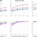
The clinicoradiomic nomogram, which integrated imaging features and clinical characteristics via logistic regression, demonstrated superior predictive performance in the validation set, with an area under the curve (AUC) of 0.936 (95% CI: 0.885–0.986), surpassing both clinical (AUC = 0.924; 95% CI: 0.873–0.976) and radiomic models (AUC = 0.828; 95% CI: 0.738–0.918) alone. Decision curve analysis further confirmed the clinical utility of this model, particularly in differentiating between gouty and non-gouty arthritis.
Conclusion
Compared with standalone clinical or radiomic models, the ultrasonography-based clinicoradiomic model exhibited enhanced predictive accuracy for diagnosing gouty arthritis, presenting a novel and promising approach for the early diagnosis and management of gouty arthritis.
Introduction
Gouty arthritis (GA) is a crystal-induced inflammatory joint disease that has seen a significant rise in incidence over recent decades [ ]. The hallmark pathological feature of GA is the deposition of monosodium urate (MSU) crystals in joints and surrounding tissues, which subsequently incites inflammatory responses and tissue damage [ , ]. This condition often affects multiple joints and, in severe cases, can lead to a loss of joint function, markedly diminishing quality of life for affected individuals. Early and accurate diagnosis is essential for the effective treatment of GA as it significantly reduces the risk of adverse outcomes [ ]. Although the current gold standard for diagnosis is the microscopic identification of MSU crystals, this method is invasive and poses challenges for routine clinical use, particularly when aspirating synovial fluid from small joints [ , ].
Ultrasonography has become the preferred diagnostic tool for GA due to its advantages that include low cost, safety, accessibility and the absence of radiation [ ]. A multi-joint controlled study by Norkuviene et al. found that ultrasound findings are of significant value in diagnosing GA, particularly the double-track sign, with a sensitivity of 84% and specificity of 81% [ ]. Naredo et al. found that the sensitivity and specificity of specific ultrasound signs for GA were 84.6% and 83.3%, respectively [ ]. However, in cases where patients present with atypical ultrasonographic features of joint pain, the diagnosis heavily relies on the operating physician’s experience, which can introduce variability. With the rapid advancement of modern medical imaging technologies, radiomics has emerged as a powerful tool that enables the extraction of high-throughput features from medical images, thereby converting image data into quantifiable and analyzable information [ ]. Radiomics can automatically extract high-dimensional features from images that are often imperceptible through visual assessment. Given its high accuracy and applicability in differential diagnosis and prognostic prediction, the potential of radiomics in the medical field is increasingly being recognized [ ]. However, there remains a paucity of research on the application of machine learning methods and radiomics in the diagnostic evaluation of GA.
This study aims to integrate machine learning algorithms, radiomic features and clinical variables to develop and validate an efficient diagnostic model for GA, with the goal of enhancing diagnostic accuracy and efficiency.
Materials and methods
Patients
Study population: We retrospectively analyzed 604 patients presenting with joint pain between June 2020 and December 2023. The cohort included 486 patients diagnosed with GA (GA group) and a control group (non-GA group) of 118 patients, comprising 88 individuals with rheumatoid arthritis (RA) and 30 with osteoarthritis (OA).
RA and OA were included in the control group for comparison with GA because they are common types of arthritis that may present with similar symptoms such as joint pain and swelling, which can lead to misdiagnosis. Furthermore, as this was a single-center study, RA and OA were the most frequently collected cases at our center, while other types of inflammatory arthritis were rare. Therefore, the non-GA group was limited to RA and OA.
Inclusion criteria:
- 1)
GA patients met the 2015 American College of Rheumatology (ACR)/European League Against Rheumatism (EULAR) gout classification criteria
- 2)
RA and OA patients conformed to the 2010 ACR/EULAR classification criteria and the “Chinese Guidelines for the Diagnosis and Treatment of Osteoarthritis” (2010 edition)
- 3)
No symptomatic treatment for arthritis within the past 6 mo
- 4)
Clear ultrasonographic images with complete data
Exclusion criteria:
- 1)
History of trauma to the evaluated joint
- 2)
Presence of malignancies
- 3)
Pregnancy or lactation
The workflow of this study is detailed in Figure S1 . We collected ultrasonography data along with demographic and clinical variables including gender, age, disease duration, body mass index, serum uric acid, serum creatinine, C-reactive protein, erythrocyte sedimentation rate, renal stones, hypertension and diabetes history. The recruitment process is detailed in Figure 1 .

This study, a retrospective analysis of imaging and clinical data, was approved by the ethics committee and the requirement for informed consent was waived. The study adhered to the principles of the Helsinki Declaration, and all patient-identifiable information was anonymized.
Methods
Ultrasound image acquisition
Ultrasound examinations were conducted using the Aiexplorer (SuperSonic Imagine, Aix-en-Provence, Cedex, France) with a linear probe L15-4 (frequency 4–15 MHz) or the Philips EPIQ7 (Philips Healthcare, Amsterdam, The Netherlands) ultrasound system with a linear probe L12-5 (frequency 5–12 MHz). The musculoskeletal imaging mode was selected and optimal depth was adjusted according to the target joint for scanning. All examinations were performed by a single experienced musculoskeletal ultrasonographer blinded to clinical data. The joint with the most pronounced symptoms was assessed in each patient, including the metatarsophalangeal, ankle, knee, elbow, wrist, shoulder and hand joints. Ultrasound examination procedures adhered to EULAR guidelines for musculoskeletal ultrasound. All images meeting inclusion and exclusion criteria were exported from the ultrasound device and reviewed by a musculoskeletal ultrasound expert.
Region of interest delineation
All included ultrasound images were re-sampled to ensure uniform pixel spacing and consistent resolution across all images. Re-sampling adjusted the images to a standardized spatial resolution of 1 mm × 1 mm to reduce variations caused by differences in acquisition settings. The re-sampling process was performed using bi-linear interpolation to preserve image quality and avoid introducing artifacts. Two imaging technicians, certified by the Chinese Academy of Management Science, manually delineated the regions of interest (ROIs) using ITK-SNAP software. These technicians were blinded to the clinical data and ultrasound diagnostic results. Following ROI delineation, the images were analyzed, and relevant features were extracted.
Feature extraction
Radiomic features were automatically extracted using the open-source Python package Pyradiomics ( https://pyradiomics.readthedocs.io/ ). These manually crafted features were divided into three categories: (i) Shape features, which describe the 2-D geometric characteristics of the ROI, such as area, perimeter and compactness; (ii) intensity features, which represent the first-order statistical distribution of pixel intensities within the ROI; and (iii) texture features, which capture patterns and higher order spatial relationships of intensity. Texture features were derived using methods such as Gray-Level Co-occurrence Matrix, Gray-Level Run Length Matrix, Gray-Level Size Zone Matrix and Neighborhood Gray-Tone Difference Matrix.
Feature selection
Statistics. Mann-Whitney U tests were performed on all radiomic features, with only those features achieving a p value < .05 being retained.
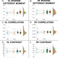
Correlation. For highly reproducible features, Spearman’s rank correlation coefficient was used to assess inter-feature correlations. If any two features exhibited a correlation coefficient greater than 0.9, only one of the correlated features was retained. Figure 2 illustrates the percentage of each group of imaging features relative to the total feature set. To maximize the retention of informative features, a greedy recursive deletion strategy was employed, wherein the most redundant feature in the current set was iteratively removed. This process resulted in the retention of 11 features.

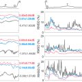
Least absolute shrinkage and selection operator. The least absolute shrinkage and selection operator (LASSO) regression model was applied to the discovery dataset to construct a signature. LASSO penalizes regression coefficients based on a regularization parameter λ, shrinking coefficients toward zero and setting many irrelevant ones to zero. To determine the optimal λ, 10-fold cross-validation using the minimum criteria was conducted, selecting the λ value that minimized cross-validation error. The retained features with non-zero coefficients were used to fit the regression model and combined into a radiomics signature. A radiomics score for each patient was then calculated as a linear combination of the retained features, weighted by their model coefficients. LASSO regression modeling was performed using the Python scikit-learn package.
Radiomics signature
Following LASSO feature selection, the final set of features was input into various machine learning models, including logistic regression (LR), support vector machines (SVM), random forest and XGBoost, to construct risk prediction models. Fivefold cross-validation was employed to derive the final radiomics signature. To assess the added prognostic value of the radiomics signature in conjunction with clinical risk factors, a radiomics nomogram was developed using the validation dataset. This nomogram integrated the radiomics signature with clinical risk factors through LR analysis. A calibration curve was then generated to evaluate concordance between the nomogram’s predictions and actual outcomes.
Clinical signature
The process of constructing the clinical signature mirrored that of the radiomics signature. Initially, clinical features were selected based on baseline statistical analysis, retaining those with p < .05. The same machine learning models used for the radiomics signature were then applied. To ensure a fair comparison, fivefold cross-validation and a fixed test cohort were utilized.
Radiomic nomogram
The radiomic nomogram was developed by integrating radiomics and clinical signatures. The diagnostic performance of the nomogram was assessed in the test cohort, with receiver operating characteristic curves generated to evaluate its diagnostic accuracy. Calibration curves were drawn to assess the nomogram’s calibration efficiency, and the Hosmer-Lemeshow goodness-of-fit test was employed to evaluate its calibration ability. Decision curve analysis (DCA) was conducted to assess the clinical utility of the predictive models.
Data sets
All patients were randomly divided into training and test groups in a 4:1 ratio. The Mann-Whitney U-test, t -test and χ² test were used to compare clinical characteristics between the two groups, identifying any significant differences in patient demographics, clinical presentation and other relevant factors that could influence study outcomes.
Results
Patients
This study retrospectively collected data from 681 patients with joint pain, excluding 28 cases of previous joint trauma, 26 cases of concomitant arthritis and 23 cases of concomitant malignancy. Ultimately, 604 patients were included, comprising 486 GA patients (GA group), 88 RA patients and 30 OA patients (non-GA group). Patients were randomly assigned to a training group (n = 483) and a validation group (n = 121). The baseline clinical characteristics of the cohort are summarized in Tables 1 and S1 .
| Feature name | Train-label = ALL | Train-label = 0 | Train-label= 1 | p value | Test-label = ALL | Test-label = 0 | Test-label = 1 | p value |
|---|---|---|---|---|---|---|---|---|
| Age | 50.41 ± 18.54 | 59.99 ± 14.90 | 48.10 ± 18.61 | <0.001 | 52.40 ± 18.07 | 59.50 ± 12.54 | 50.65 ± 18.84 | 0.022 |
| BMI | 25.57 ± 3.30 | 23.00 ± 3.34 | 26.19 ± 2.97 | <0.001 | 25.50 ± 3.53 | 23.07 ± 3.17 | 26.10 ± 3.36 | <0.001 |
| High blood pressure | 0.32 ± 0.61 | 0.31 ± 0.99 | 0.33 ± 0.47 | 0.061 | 0.36 ± 0.48 | 0.33 ± 0.48 | 0.36 ± 0.48 | 0.759 |
| Course | 35.36 ± 58.55 | 44.17 ± 73.78 | 33.23 ± 54.13 | 0.037 | 33.43 ± 47.63 | 42.00 ± 43.95 | 31.31 ± 48.48 | 0.090 |
| Kidney stones | 0.31 ± 0.46 | 0.09 ± 0.28 | 0.37 ± 0.48 | <0.001 | 0.32 ± 0.47 | 0.08 ± 0.28 | 0.38 ± 0.49 | 0.005 |
| Creatinine | 91.52 ± 68.96 | 68.31 ± 16.17 | 97.12 ± 75.39 | <0.001 | 87.00 ± 40.38 | 60.08 ± 17.70 | 93.66 ± 41.67 | <0.001 |
| Uric acid | 448.24 ± 127.69 | 327.69 ± 84.51 | 477.37 ± 119.05 | <0.001 | 423.60 ± 136.78 | 298.92 ± 83.47 | 454.44 ± 129.88 | <0.001 |
| CRP | 31.19 ± 49.90 | 37.07 ± 47.00 | 29.76 ± 50.53 | 0.036 | 30.79 ± 44.45 | 23.71 ± 21.98 | 32.54 ± 48.35 | 0.778 |
| ESR | 38.91 ± 38.07 | 53.79 ± 35.38 | 35.31 ± 37.87 | <0.001 | 35.76 ± 32.27 | 50.83 ± 29.96 | 32.04 ± 31.87 | 0.004 |
| Gender | <0.001 | <0.001 | ||||||
| Female | 84 (17.39) | 56 (59.57) | 28 (7.20) | 27 (22.31) | 18 (75.00) | 9 (9.28) | ||
| Male | 399 (82.61) | 38 (40.43) | 361 (92.80) | 94 (77.69) | 6 (25.00) | 88 (90.72) | ||
| Diabetes | 0.024 | 1 | ||||||
| 0 | 408 (84.47) | 87 (92.55) | 321 (82.52) | 98 (80.99) | 19 (79.17) | 79 (81.44) | ||
| 1 | 75 (15.53) | 7 (7.45) | 68 (17.48) | 23 (19.01) | 5 (20.83) | 18 (18.56) | ||
| Cardiovascular diseases | 0.27382 | 0.964103 | ||||||
| 0 | 406 (84.06) | 83 (88.30) | 323 (83.03) | 103 (85.12) | 21 (87.50) | 82 (84.54) | ||
| 1 | 77 (15.94) | 11 (11.70) | 66 (16.97) | 18 (14.88) | 3 (12.50) | 15 (15.46) |
Related posts:
 Advances in the Application of Artificial Intelligence in the Ultrasound Diagnosis of Vulnerable Carotid Atherosclerotic Plaque
 Changes in Muscle Quality Following Short-Term Resistance Training in Older Adults: A Comparison of Echo Intensity and Texture Analysis
 Guided-VCTE: An Enhanced FibroScan Examination With Improved Guidance and Applicability
 Regional Image Quality Scoring for 2-D Echocardiography Using Deep Learning
 Ultrafast Coherence-Based Power Doppler Estimation Using Nonlinear Compounding With Complementary Subset Transmit
 Near-Field Clutter Mitigation in Speckle Tracking Echocardiography
Stay updated, free articles. Join our Telegram channel

Full access? Get Clinical Tree


