Abstract
Objective
The current diagnosis of salivary gland tumors (SGTs) is dependent on subjective ultrasound features. Here we aimed to develop an objective method using ultrasound radiomics.
Methods
We collected 248 benign and 46 malignant images and divided them into training (80%) and testing (20%) groups, with 105 radiomic features extracted from each image. Data re-sampling, feature selection and classification were conducted. The diagnostic accuracy of different combinations was evaluated.
Results
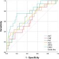
After data re-sampling using the Synthetic Minority Over Sampling Technique (SMOTE) and feature selection with LASSO+ANOVA, 10 radiomic features were selected. Using the Random Forest classifier, the testing set achieved an area under the receiver operating characteristic curve of 0.85, accuracy of 90%, sensitivity of 78% and specificity of 92% for diagnosing SGTs. It maintained an accuracy of 85% in a separate internal validation set.
Conclusion
This study offers significant insights into the use of radiomics for the diagnosis of SGTs. When selected properly and paired with a suitable classification model, radiomics can be used to differentiate between benign and malignant SGTs.
Introduction
Salivary gland tumors (SGTs) encompass benign and malignant tumors, and each exhibits distinct behaviors. Accurate diagnosis through imaging examinations can be challenging [ ] and the management approach varies significantly between benign and malignant SGTs, requiring different surgical procedures [ ]. To ensure proper SGT management, pre-operative procedures such as fine-needle aspiration (FNA) and/or core needle biopsy (CNB), or intra-operative frozen section analysis, are often employed to determine the benignity or malignancy of SGTs [ ]. However, complications such as tumor seeding and transient facial paralysis may occur [ ].
With advancements in technology, ultrasound (US) has been widely used for evaluating various head and neck tumors, including SGTs [ ]. Clinicians can diagnose these tumors as benign or malignant based on specific US image features. Previously we developed a subjective US model for diagnosing malignant SGTs [ , ]. However, the subjective interpretation of US images can lead to diagnostic disagreements. Additionally, there is currently no objective method for reporting US images of SGTs. Therefore, in this study we wished to establish an objective method to assist in the diagnosis of SGTs using US images.
To address the limitations of subjective US feature methods, we utilized radiomics and machine learning (ML) [ , ]. Radiomics extracts quantitative features from medical images using mathematical analysis [ ] that are derived from the spatial distribution of signal intensity within images and can reveal disease characteristics that may elude the naked eye. The process of using radiomics and ML for image classification involves several steps. First, the region of interest (ROI) in the image is selected. Next, radiomic features are extracted from the chosen ROI and ML models are used to select the most important features. Finally, a model is constructed using the selected features to perform image classification.
Currently, software for extracting radiomic features includes MATLAB and PyRadiomics [ ]. Most studies using radiomics and ML in the head and neck region focus on thyroid tumors [ , ], with only one article evaluating SGTs . Li et al. utilized MATLAB for ROI selection and feature extraction [ ]. They selected 26 radiomic features using LASSO and achieved an area under the receiver operating characteristic curve (AUC) of 0.80 using linear regression. However, MATLAB’s annual cost of around USD1000 may not be feasible for every hospital. Alternatively, PyRadiomics is an open-source Python package. Our study employed 3-D Slicer, an open-source software equipped with PyRadiomics, for ROI delineation and feature extraction. This software offers a user-friendly interface for segmentation and feature selection, and has more functionality than MATLAB, with over 300 modules and extensions [ ]. It can also integrate with other imaging tools, greatly facilitating the process of ROI selection and radiomic feature extraction.
In this study, we aimed to review and analyze US images of patients with SGTs. We planned to extract radiomic features from these images, select the most relevant features and construct a classification model using various ML models. Our goal was to develop an objective method for diagnosing SGTs using radiomics and ML techniques, all within the framework of open-source software.
Methods
Ethical considerations
This study, which is retrospective in nature, was approved by the Institutional Review Board (IRB no. 111199-E and 112136-E). It adhered to the Declaration of Helsinki and complied with the CheckList for EvaluAtion of Radiomics Research (CLEAR).
Inclusion criteria
This study was carried out at a tertiary medical center and we examined the records of patients who visited the out-patient department between January 2007 and December 2021 for SGTs. Our study included adult patients who had undergone US examinations and additional operations or CNBs. Head and neck USs were conducted by two experienced otolaryngologists with over a decade of practice. A Toshiba Aplio 500 (Canon Medical Systems, Tochigi-ken, Japan) was used, which is equipped with a 5–14 MHz linear-array transducer. CNB was carried out when patients were considered unsuitable for open surgery or when they opted against open surgery. Pathological diagnosis, derived from pathological reports, served as the definitive reference for classifying tumors as either malignant or benign. Patients with poor-quality US images were excluded from the study.
Data collection
In this study a total of 294 patients with SGTs were included, 248 of whom had benign tumors and 46 who had malignant tumors. For each patient we collected a single representative US image, specifically the one that depicted the longest axis. These US images were retrieved from the Picture Archiving and Communication System. To maintain patient confidentiality, we removed all identifiable information from the US images, including names, birth dates, admission dates and medical record numbers, using the Snipping Tool (Microsoft). Consequently, we amassed a collection of 248 benign and 46 malignant US images. The clinical data, which included age, gender, smoking status, tumor side, location and size, as well as pathological confirmation and diagnoses, were also collected in this study.
Segmentation and feature extraction
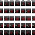
We utilized 3-D Slicer, an open-source medical imaging software equipped with a PyRadiomics package, to select the ROI ( Fig. 1 ). This software facilitates the selection of ROIs and extraction of radiomic features. ROI selection was performed by two seasoned otolaryngologists, each with over 10 y of experience in US practice. They employed manual segmentation techniques, with each checking the other’s work. No disagreement in ROI selection was reported. All 2-D features were extracted from the original US images using PyRadiomics and no image filters were applied in our study.

Number of extracted features
From each of the 296 US images, 105 radiomic features were collected. Subsequently, these images were randomly divided into a training set (235/294, 80%) and a testing set (59/294, 20%). Given the evident data imbalance between benign and malignant cases (248:46), we resampled the training set using ML techniques such as Random Under Sampling (RUS), Random Over Sampling (ROS) and Synthetic Minority Over Sampling Technique (SMOTE) [ ]. These data re-sampling methods balanced both classes by generating new data for the minor class through random duplication (ROS), synthesizing new instances by interpolating among existing samples of the minority class (SMOTE) or reducing the size of majority class via random deletion (RUS). Considering the wide range of these 105 radiomic features, we standardized the training set, resulting in data with a mean value of 0 and a standard deviation of 1. The same standardization was subsequently applied to the testing set.
Feature categories
The 105 radiomic features could be categorized into seven groups [ , ]:
- 1.
Shape-based features (n = 12): These features described the 2-D size and shape of the ROI.
- 2.
First-order statistics features (n = 18): These features characterized the distribution of pixel intensities within the ROI.
- 3.
Gray Level Co-occurrence Matrix (GLCM) features (n = 24): These features captured spatial relationships between adjacent pixels.
- 4.
Gray Level Dependence Matrix (GLDM) features (n = 14): These features quantified the dependence of pixel values by assessing the number of adjacent pixels with the same gray level as the central pixel.
- 5.
Gray Level Run Length Matrix (GLRLM) features (n = 16): These features analyzed the length of runs of pixel values by calculating the number of consecutive pixels with the same gray level in a specific direction.
- 6.
Gray Level Size Zone Matrix (GLSZM) features (n = 16): These features quantified gray level zones, defined as the number of connected voxels with the same gray level.
- 7.
Neighboring Gray Tone Difference Matrix (NGTDM) features (n = 5): These features quantified differences in neighboring pixel intensities.
Feature selection and model establishment
After extracting the radiomic features and pre-processing the data, we employed various ML models for feature selection. These included filter methods (such as ANOVA), wrapper methods (such as recursive feature elimination [RFE]), embedded methods (such as LASSO regression, ElasticNet, Linear Support Vector Classifier [SVC] with L1 penalty) and tree-based methods (such as Random Forest classifier and Extra Trees classifier, both with feature importance) to identify the most relevant features [ ]. Subsequently, we established a diagnostic model using binary classification ML models, including logistic regression, SVC, linear SVC, K-nearest neighbors classifier, Decision Tree classifier, Random Forest classifier and Extra Trees classifier [ , ]. We conducted all possible combinations of data re-sampling, feature selection and binary classification method establishment. All of these steps, encompassing data pre-processing, feature selection and binary classification model development, were executed within the Python framework on Google Colaboratory (Colab), an online Jupyter Notebook platform.
Statistical analysis
A confusion matrix was generated that included measures such as accuracy, sensitivity, specificity, positive-predictive value and negative-predictive value, along with AUC. Sensitivity and specificity pertain to the diagnosis of malignant SGTs. These metrics were obtained by applying the model to the testing set. The model that demonstrated the highest diagnostic accuracy and AUC was selected for application.
Internal validation
After the model was established, we gathered a separate group of patients between January 2023 and June 2023 who fulfilled the same inclusion criteria. This group served as an internal validation for our model and was also assessed using the subjective US model, CT report and fine-needle aspiration cytology (FNAC). A CT report was interpreted as malignant if it reported suspicion of malignancy. An FNAC report was diagnosed as malignant if atypia or malignancy was noted.
Results
Inclusion and exclusion criteria are illustrated in Figure 2 , while the entire process for radiomic feature analysis and SGT classification is demonstrated in Figure 3 . This study gathered data from 294 patients with SGTs, who we randomly divided into a training set (235/294, 80%) and a testing set (59/294, 20%). Clinical characteristics between the training and testing sets are compared in Table 1 . The training set consisted of 198 benign and 37 malignant tumors, while the testing set included 50 benign and 9 malignant tumors. There were no significant differences in age, gender, smoking status, tumor side, tumor location, tumor size, pathological confirmation and pathological diagnoses between the training and testing sets (all p values > 0.05). Pathological reports for the training and testing sets are presented in Table 2 .


| Clinical characteristic, mean (SD) or N (%) | Training | Testing | p value |
|---|---|---|---|
| N = 235 | N = 59 | ||
| Age, y | 53 (14) | 53 (15) | 0.876 |
| Gender | 0.840 | ||
| Female | 99 (42%) | 24 (41%) | |
| Male | 136 (58%) | 35 (59%) | |
| Smoking status | 0.789 | ||
| No | 132 (56%) | 32 (54%) | |
| Yes (including quitted) | 103 (44%) | 27 (46%) | |
| Tumor side | 0.886 | ||
| Right | 125 (53%) | 32 (54%) | |
| Left | 110 (47%) | 27 (46%) | |
| Tumor location | 0.792 | ||
| Parotid gland | 183 (78%) | 45 (76%) | |
| Submandibular gland | 52 (22%) | 14 (24%) | |
| Tumor size | |||
| Long axis, cm | 2.5 (1.0) | 2.4 (1.0) | 0.509 |
| Short axis, cm | 1.7 (0.6) | 1.6 (0.6) | 0.519 |
| Short-long-axis ratio | 0.7 (0.2) | 0.7 (0.1) | 0.929 |
| Pathological confirmation | 0.797 | ||
| Operation | 221 (94%) | 56 (95%) | |
| Core needle biopsy | 14 (6%) | 3 (5%) | |
| Pathological diagnosis | 0.926 | ||
| Benign tumor | 198 (84%) | 50 (85%) | |
| Malignant tumor | 37 (16%) | 9 (15%) |
| Pathological report | Training | Testing |
|---|---|---|
| N = 235 | N = 59 | |
| Benign salivary gland tumors | 198 | 50 |
| Pleomorphic adenoma | 74 (37%) | 24 (48%) |
| Warthin’s tumor | 81 (41%) | 13 (26%) |
| Other benign tumors (basal cell adenoma, oncocytoma, hemangioma, lymphadenoma, chronic sialadenitis, IgG4-associated sialadenitis, etc.) | 43 (22%) | 13 (26%) |
| Malignant salivary gland tumors | 37 | 9 |
| Metastatic carcinoma | 9 (24%) | 2 (22%) |
| Poorly differentiated/undifferentiated carcinoma | 8 (22%) | 3 (33%) |
| Mucoepidermoid carcinoma | 7 (19%) | 1 (11%) |
| Lymphoma | 5 (14%) | 0 (0%) |
| Lymphoepithelial carcinoma | 4 (11%) | 0 (0%) |
| Adenoid cystic carcinoma | 1 (3%) | 1 (11%) |
| Adenocarcinoma | 1 (3%) | 1 (11%) |
| Carcinoma ex pleomorphic adenoma | 1 (3%) | 0 (0%) |
| Salivary duct carcinoma | 1 (3%) | 0 (0%) |
| Acinic cell carcinoma | 0 (0%) | 1 (11%) |
Related posts:
 Quantitative Analysis of Contrast-Enhanced Ultrasound Images of Brain-Dead Donor Livers: Prediction of Early Allograft Dysfunction
 Safety of Shear Wave Elastography as Evidenced From Carotid Artery Strain and Strain Rate Induced by Acoustic Radiation Force Impulse and Arterial Pulsations
 SegFormer3D: Improving the Robustness of Deep Learning Model-Based Image Segmentation in Ultrasound Volumes of the Pediatric Hip
 Ultrasound Shear Wave Elastography and Shear Wave Dispersion: Correlation with Histopathological Changes in Autoimmune Hepatitis Patients
 Clutter-Generating Phantom Material. Part II: Utilization in the Comparison of Conventional and Regularized Ultrasound Attenuation Estimation
 Low-intensity Pulsed Ultrasound Stimulation of the Intestine Improves Insulin Resistance in Type 2 Diabetes
Stay updated, free articles. Join our Telegram channel

Full access? Get Clinical Tree


