Estimation of In Vivo Human Carotid Artery Elasticity Using Arterial Dispersion Ultrasound Vibrometry

Abstract

Objective

Arterial stiffening serves as an early indicator for a variety of cardiovascular diseases. Arterial Dispersion Ultrasound Vibrometry (ADUV) is a method that leverages acoustic radiation force to stimulate arterial wall motion, assess wave propagation characteristics, and subsequently calculate the arterial shear modulus. Previously, we introduced an inversion technique based on a guided cylindrical wave model, which proved effective in rubber tube phantom experiments. In this study, we broaden the scope of our investigation from phantom experiments to in vivo examination of common carotid arteries in human subjects, identify the challenges, and provide solutions, leading to a systematic protocol for ADUV application and robust estimation of the elastic modulus of common carotid arteries.

Methods

We achieve this by analyzing ADUV data from 59 subjects categorized as (a) confirmed atherosclerotic cardiovascular disease ( n = 27), (b) with cardiovascular risk factors ( n = 20), and (c) healthy ( n = 12). A crucial aspect of this work is the development of metrics to differentiate high-quality ADUV data from unusable data.

Results and Conclusions

With the proposed metrics, in our cohort, we observed 82% of diameter data and 78% of motion data as usable data. Future work will involve applying this protocol to a larger cohort with subsequent statistical analysis to assess and validate the resulting biomarkers.

Introduction

Arterial stiffness is an early indicator for many cardiovascular diseases [ ]. The gold standard technique to measure arterial stiffness is the use of arterial pulse wave velocity (PWV), typically the carotid-to-femoral PWV (cfPWV) [ ]. However, this method experiences several limitations with the primary being inaccurate distance measurement [ ] and the requirement of long distances for time measurement due to low spatial resolution [ ]. In recent times, fast ultrasound-based Pulse Wave Imaging [ , ] has been utilized to estimate the local instantaneous pulse wave velocity measurement. However, this approach fails to provide artery stiffness distribution over the entire cardiac cycle.

While the above-mentioned methods use the endogenous pulsatile motion of the artery as an excitation source, there have been efforts to induce waves in the arterial wall by applying an acoustic radiation force (ARF) to make measurements of arterial material modulus (see [ ] for details on various ARF-based methods). Among these imaging techniques, Shear Wave Elastography (SWE) has become a promising tool because the shear modulus has a wider range than the bulk modulus for soft tissues [ ]. Several studies focused on estimating arterial stiffness using SWE; many of them focused on phantoms [ ], few of them considered in vivo data [ , ] as well using simplified inversion framework, e.g., based on group velocity, Lamb wave velocity in plates.

As mentioned in prior studies by , for the boundary-sensitive arterial waveguide problem, the generated shear waves are dispersive in nature, i.e., phase velocity changes with frequency and depends on both wall thickness and artery radius. To account for these effects, we have recently developed a physics-based arterial waveguide model based on the semi-analytical finite element method [ , ], and applied it for inverting the elastic modulus. The approach was validated with data from rubber tube phantom experiments. In this work, we extend the framework for in vivo settings, which turned out to be nontrivial with natural complexities associated with acquiring both geometry (lumen diameter and wall thickness) and wall motion data due to the applied ARF.

The primary aim of this paper is thus to provide guidelines for estimating the shear modulus of the carotid arterial wall using the Arterial Dispersion Ultrasound Vibrometry (ADUV). These are developed by performing extensive data processing with ADUV data obtained from a total of 59 subjects (a) with confirmed atherosclerotic cardiovascular disease, (b) with cardiovascular risk factors, and (c) healthy subjects. Note that our current goal is not to evaluate the validity of ADUV-based elastic modulus as a biomarker, but to develop a protocol for ADUV application (the protocol will be applied to an expanded cohort of subjects, followed by statistical analysis in future work).

Methodology

Arterial Dispersion Ultrasound Vibrometry (ADUV)

Arterial Dispersion Ultrasound Vibrometry (ADUV) estimates arterial modulus by minimizing the misfit between measured and simulated dispersion curves, i.e., phase velocity as a function of frequency. Simulated dispersion curves are obtained using an underlying analytical or computational model, referred to as the forward model. The measured dispersion curves are obtained by processing wall motion data from ultrasound. The modulus estimation is done by inverse optimization. All these steps are outlined in the remainder of the section, setting the stage for the importance of different steps of in vivo data acquisition.

Forward model

We idealize the artery to be a cylindrical tube immersed in and filled with inviscid fluid and utilize the semi-analytical finite element (SAFE) method to obtain the simulated dispersion curves. The schematic of the geometry is presented in Figure 1 a. The guided waves in the tube are obtained by solving the elastodynamic equation in the tube wall (solid domain Ω S ), coupled with its interaction with the surrounding incompressible fluid ( Ω F ). The details of the formulation can be found in [ ]; we simply summarize the main aspects here. The governing equations are thus,

−LσT(GLσu)+ρSd2udt2=0,inΩS,

where u is the displacement, and ρ S is the solid density. L σ is the symmetric gradient. Given the incompressibility and inviscid assumptions, the fluid domain inside and outside is governed by the Laplace equation,

∇2p=0inΩF,

where p is the fluid pressure. The variables u and p are governed by the traction and displacement continuity conditions at the solid-fluid interfaces Γ F S :

(GLσu)·ns−pnF=0,onΓFS,

ρFd2udt2·ns−∂p∂nF=0,onΓFS,

where ρ F is the fluid density and n s , n F are the unit vectors in the solid and fluid domains respectively, which are opposites of each other.

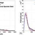
While Equations (1)–(4) are 3D partial differential equations, they are efficiently solved with the help of a semi-analytical finite element (SAFE) framework. Particularly, we use the harmonic solutions in the axial ( x ) , circumferential ( θ ) , directions of the tube, and time ( t ) direction while the finite element discretization is applied in the radial ( r ) direction only. This results in an algebraic eigenvalue problem relating the wavenumber to frequency, which is then solved to obtain the final dispersion relations for multiple wave modes ( Fig. 1 b). The details of our SAFE framework, which includes additional efficiencies aided by special discretization techniques (Selective Reduced Integration scheme [ ] and Perfectly Matched Discrete Layers for the absorbing boundary conditions [ , ]) can be found in [ ].

Note that we consider only the elasticity of the arterial wall. As observed by [ ] and [ ], the phase velocity dispersion curves are not significantly sensitive to the viscosity due to the presence of the geometric dispersion in the considered frequency range.

Inverse model

The forward model described in the previous section results in the dispersion curves given the radius of the lumen, the thickness of the wall, densities of both the wall and the surrounding fluid, and the shear modulus of the wall. The inverse model aims at estimating some of the parameters from the observed dispersion curves. To make the process well-posed, it would be prudent to minimize the number of parameters to invert, while maximizing their sensitivities. Given this, we assume the standard values of the arterial and fluid density (1000 kg/m ³ ), obtain the geometric measurements from ultrasound B-mode imaging and simply invert just for the elastic modulus, specifically the shear modulus, which is our current focus. It should be noted that viscoelasticity can be inverted too, but from full-wave response and not from the dispersion curves [ ]. While our previous work demonstrated the effectiveness of the full-wave inversion method for estimating arterial viscoelasticity using in silico data, further work is needed before in vivo applications, e.g., validating with phantom and/or ex vivo experiments. Therefore, in this study, we focus on estimating the elastic component of the shear modulus for which dispersion matching is a robust approach.

Our goal is to estimate the unknown shear modulus of the arterial wall by minimizing the misfit between measured and simulated dispersion curves. The method has been developed in [ ], which included validation with rubber tubes. In that work, we found that this forward model is utilized in inverting rubber tube data, where we observed that different wave modes (F [1,1] and F [2,1]) dominate at different frequency ranges (900–1000 Hz and 300–500 Hz, respectively), which lead us to advocate for matching different modes for different frequency windows. Unfortunately, for in vivo settings, we found that the noise is more significant, and it is difficult to obtain reliable dispersion curves at higher frequencies. In this study, we will restrict ourselves to match the dispersion curves for the F (1,1) mode for the lower frequency range of 250–500 Hz. The inverse problem can then be stated as finding the value of the shear modulus that minimizes the objective function defined as the least-squares difference between the measured and simulated phase velocities:

G0=argminG[∑fi=250Hz500Hz(c1s(fi,G0)−cm(fi))2],

where G 0 is the inverted shear modulus, c 1 s ( f , G ) is the simulated phase velocity for F (1,1) mode and c m is the measured phase velocity obtained from the measured motion data (details are in the following Section Computation of phase velocity dispersion). The inverse problem can be solved by formulating a partial differential equation-constrained optimization problem with explicit expressions of gradient and Hessian by utilizing an adjoint operator. Such an approach is beneficial for a large number of inversion parameters. Given that we have only one parameter, we use the finite difference method with a relative step size of 1 × 10 ^-5 to compute the gradient, and the BFGS (Broyden–Fletcher–Goldfarb–Shanno) method through the MATLAB fmincon function, to perform the optimization for the objective function in Equation (5) . We also impose minimum and maximum values of G 0 as 50 kPa and 800 kPa, respectively. With respect to the runtime, the inversion took around 1.5 seconds on a standard desktop computer (Intel® Core(TM) i7-6700 CPU, 3.40 GHz with 32.0 GB RAM and 64-bit OS).

Examining the optimization problem in Equation (5) , it is important to have (a) accurate radius/diameter and thickness to compute the simulated phase velocities c 1 s , and (b) accurate particle velocities and associated data processing to obtain the measured phase velocities c m . These details are discussed in the remainder of the section.

Measuring radius and thickness

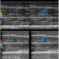
Lumen diameter and wall thickness can be obtained from either longitudinal or transverse B-mode images of the common carotid artery (CCA). The challenge in utilizing the longitudinal B-mode image is ensuring that the scanning plane accurately traverses the center of the vessel. Misalignment can introduce errors, especially in diameter measurement, consequently affecting the accuracy of the inverted modulus. This problem is addressed by using a transverse imaging in which the transverse B-mode cines of the common carotid artery (CCA) are recorded over the course of multiple cardiac cycles and saved as DICOM files using a clinical ultrasound scanner (GE LOGIQ E9 and GE LOGIQ E10, General Electric Healthcare, Wauwatosa, WI) with a 2–9 MHz linear array probe at a frame rate between 30 and 50 Hz, pixel spacing 0.04–0.08 mm, and image matrix sizes of either 802 × 1054 pixels (LOGIQ E10) or 519 × 680 pixels (LOGIQ E9). The transverse view is then chosen to ensure that the full diameter of the vessel is imaged.

A custom semiautomated retrospective M-mode approach is used to extract the diameter waveform of the CCA from each cine. DICOM files are loaded into MATLAB (R2021a, MathWorks, Natick, MA). The first frame of each cine is used to manually identify the location and place approximate upper and lower bounds for the diameter. A patch of the first frame centered about the CCA is then manually defined and extracted, and the MATLAB function normxcorr2 is used to find reduced-size regions of interest (ROIs) in each subsequent frame that are most closely correlated with this image patch.

The center coordinates of circular features whose diameters fall within the previously defined diameter bounds are identified using a circular Hough transform (MATLAB function imfindcircles , sensitivity factor = 0.99, edge threshold = 0.22). For frames with multiple detected circles, the center is selected as the one closest to the mean center, across temporally adjacent frames. For frames where no circle is detected, spline interpolation using center coordinates in temporally adjacent frames is applied to estimate the location of the center in that frame.

Subsequently, a 0.6 mm wide image column at the estimated center is retrieved from each frame, and a row-wise minimum filter is applied to extract the longest anechoic region, i.e., the inner diameter of the CCA. This axial profile from each frame is plotted against time to obtain an M-mode view of the pulsating vessel. A global threshold is set manually to separate the anechoic lumen from the echogenic tissue and obtain a binarized image of the lumen over time. This image is median filtered (MATLAB function medfilt2 , 3 × 3 pixel neighborhood), and at each time point, the longest connected anechoic region within this mask is taken to be the inner diameter of the vessel lumen (see Fig. 2 ).

The above approach measuring the diameter approach relies primarily on image data along the axial direction of the transducer rather than the lateral direction. We chose to privilege axial measurements for two reasons. First, ultrasound imaging has substantially improved resolution in the axial direction compared to the lateral direction. Second, the lumen-intima interfaces corresponding to the interior diameter of the CCA appear most prominent along the axial direction and are absent laterally (see Fig. 3 ).

The diameter measurements across multiple cardiac cycles ( Fig. 4 a, black curve), are filtered to obtain a diameter history that repeats for each cardiac cycle. This is performed with a Fourier series expansion of the history and selecting only the terms with the first two multiples of the cardiac frequency (resulting in the blue curve in Fig. 4 a, which is periodic with respect to the cardiac cycle).

The thickness is measured using the longitudinal B-mode images at the peak of the R-wave of the ECG signal (cardiac stage 1) when the thickness is maximum compared to the other cardiac stages. This thickness spans the intima to media of the carotid artery, and the borders are automatically detected by the clinical scanner and may be adjusted by the sonographer [ ]. Once the thickness at cardiac stage 1 is accurately measured, the thickness at other cardiac stages (explained below related to the ARF application) is obtained from the diameter measurements at those cardiac stages, using the notion that the cross-sectional area of the artery remains constant due to the incompressibility of the tissue. Figure 4 b presents the example results for the computed thickness over the cardiac cycle (orange curve), along with the diameter variation (blue curve, obtained from the filtered history shown in Fig. 4 a).

Accepting diameter data

To assess the quality of diameter measurements, we use the root mean square error ( RMSE ) between the measured data ( d m , the black curve in Fig. 4 a), and filtered curve ( d f , the blue curve in Fig. 4 a): considering the history from the first peak to the last peak. We consider the diameter measurement to be acceptable when R M S E ≤ 5 % , which resulted in around an 82% acceptance rate across all the measurements from the 59 subjects. Figure 5 shows three representative cases for good, marginally accepted, and rejected cases.

RMSE=Mean((dm−df)2)Mean(dm2),

Only gold members can continue reading. Log In or Register to continue