Interactively Fusing Global and Local Features for Benign and Malignant Classification of Breast Ultrasound Images

Abstract

Objective

Breast ultrasound (BUS) is used to classify benign and malignant breast tumors, and its automatic classification can reduce subjectivity. However, current convolutional neural networks (CNNs) face challenges in capturing global features, while vision transformer (ViT) networks have limitations in effectively extracting local features. Therefore, this study aimed to develop a deep learning method that enables the interaction and updating of intermediate features between CNN and ViT to achieve high-accuracy BUS image classification.

Methods

This study introduced the CNN and transformer multi-stage fusion network (CTMF-Net) consisting of two branches: a CNN branch and a transformer branch. The CNN branch employs visual geometry group as its backbone, while the transformer branch utilizes ViT as its base network. Both branches were divided into four stages. At the end of each stage, a proposed feature interaction module facilitated feature interaction and fusion between the two branches. Additionally, the convolutional block attention module was employed to enhance relevant features after each stage of the CNN branch. Extensive experiments were conducted using various state-of-the-art deep-learning classification methods on three public breast ultrasound datasets (SYSU, UDIAT and BUSI).

Results

For the internal validation on SYSU and UDIAT, our proposed method CTMF-Net achieved the highest accuracy of 90.14 ± 0.58% on SYSU and 92.04 ± 4.90% on UDIAT, which showed superior classification performance over other state-of-art networks ( p < 0.05). Additionally, for external validation on BUSI, CTMF-Net showed outstanding performance, achieving the highest area under the curve score of 0.8704 when trained on SYSU, marking a 0.0126 improvement over the second-best visual geometry group attention ViT method. Similarly, when applied to UDIAT, CTMF-Net achieved an area under the curve score of 0.8505, surpassing the second-best global context ViT method by 0.0130.

Conclusion

Our proposed method, CTMF-Net, outperforms all existing methods and can effectively assist doctors in achieving more accurate classification performance of breast tumors.

Introduction

Breast cancer has become one of the primary cancers threatening women’s health and lives [ ], and early screening and diagnosis are crucial for successful treatment [ ]. Breast imaging techniques are widely used for early screening and diagnosis, including mammograph, ultrasound and magnetic resonance imaging [ ]. Among these techniques, ultrasound has advantages of having non-ionizing radiation, being non-invasive and portable, and imaging in real time. It generates breast ultrasound (BUS) images that provide crucial information for the diagnosis and classification of benign and malignant tumors. However, current BUS classification heavily relies on subjective expertise, resulting in variability. Therefore, automatic classification methods are important to reduce subjectivity, improve diagnostic accuracy and ensure consistency.

Numerous traditional methods have been used for automatic BUS classification, including linear classifiers [ ], support vector machines [ ], K-nearest neighbors [ ], decision tree [ ] and artificial neural network [ ]. However, their reliance on manual feature selection has limited their accuracy and resulted in reduced robustness [ ].

In recent years, deep learning methods have gained popularity in BUS diagnostics [ ], which can be categorized into convolutional neural network (CNN)-based methods and transformer-based methods. CNN-based methods have been extensively applied in various image classification tasks, including BUS classification. In 2022, Lu et al. [ ] utilized a pre-trained ResNet-18 with spatial attention and introduced SAFNet to enhance BUS classification, achieving 94.10% accuracy on the BUSI dataset, which is an enhancement of 4.1% over the second best cancer diagnosis model, the shallow-deep CNN [ ], also discussed in their paper. In the same year, Xi et al. [ ] developed a modality correlation-embedding network to improve the fusion of BUS images and mammography, reaching 95% accuracy. In summary, these CNN-based methods excel at extracting local features without the need for manual feature selection and have demonstrated good performance. However, their receptive range remains limited due to the constraints of convolutional kernel size, making them less adept at capturing global features [ ].

Transformer-based methods, primarily the vision transformer (ViT), have been proposed and utilized for image classification, including BUS classification. By leveraging the self-attention mechanism of the transformer structure, ViT can adaptively focus on different areas of an image, thereby extracting global features and capturing long-distance dependencies between different regions of the image. In 2020, Dosovitskiy et al. [ ] introduced ViT and applied it to image classification tasks, which surpassed the performance of the most advanced CNN networks at that time. In 2021, Gheflati et al. [ ] applied ViT to BUS classification, achieving 86.7% accuracy and an area under curve (AUC) of 0.95, outperforming the state-of-the-art CNN-based approaches [ ] in classification performance. In 2022, Gelan and Se-woon [ ] developed a multi-stage transfer-learning method using ViTs for breast cancer detection, achieving 92.8% accuracy on the BUSI dataset. While the ViT network is effective at extracting global features, it may not be as proficient as CNNs at extracting local features from images [ ]. Moreover, the ViT network may not perform as well as CNNs on tasks with small datasets such as BUS image classification [ ].

CNN-based methods excel at capturing local image features, while transformer-based methods are adept at capturing global features. Combining CNN and transformer methods can leverage the advantages of both. In 2021, Liu et al. [ ] introduced the CVM-Cervix framework for cervical cell classification, achieving fusion by concatenating the output features of the two streams. This method achieved a superior accuracy of 91.72%, outperforming other CNN and transformer-based approaches. In 2023, Maurya et al. [ ] introduced a cervical cell classification method that integrated MobileNet and ViT with features that concatenated prior to the output, achieving 97.65% accuracy. Li et al. [ ] proposed a multi-scale attention fusion module to merge the outputs of CNN and transformer encoders for thyroid nodule segmentation that achieved an 82.65% dice co-efficient. However, these previous combination methods [ ] have simply merged features after separate CNN and transformer extraction processes. Due to distinct feature extraction processes and a lack of interaction among intermediate features, CNNs and transformers may produce notably different features [ ]. Therefore, simply merging features potentially limits feature fusion and BUS classification performance [ ].

To address the limitations of the aforementioned simple fusion techniques, here we propose a CNN and transformer multi-stage fusion network (CTMF-Net) for BUS classification. This network enables the interaction and fusion of intermediate features from both the CNN and transformer extraction processes. Within CTMF-Net, its CNN and transformer branches are divided into four stages, and a feature interaction module (FIM) is proposed for feature interaction and fusion after each stage. The FIM employs a cross-attention mechanism to gauge the mutual influence between intermediate features and fuse them accordingly. Additionally, the feature extraction capability of the CNN stage is enhanced by integrating the convolutional block attention module (CBAM) [ ]. Our main contributions are as follows:

1)

We proposed a new network that integrates the CNN and transformer through multi-level interactive fusion, namely CTMF-Net, for the classification of benign and malignant tumors in BUS images. This network can improve classification performance through interactive feature representation learning.
2)

We designed a new interactive intermediate feature fusion module that enables the interaction and updating of intermediate features between the CNN and transformer.
3)

Extensive experiments on three public BUS datasets show that our method consistently improved the accuracy of breast tumor classification.

Materials and methods

Dataset

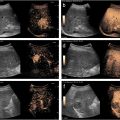
In this study, we utilized three datasets for validation. Table 1 shows a summary of all the datasets used in this study. SYSU is a publicly available BUS dataset from the Sun Yat-sen University Cancer Center (Canton, China) [ ]. This dataset has been restructured [ ] and consists of 980 samples. All samples were acquired using an iU22 xMATRIX scanner (Philips, USA) or a LOGIQ E9 scanner (GE, USA). The input of each sample was a BUS image, while the output label was derived from the patient’s pathological findings. SYSU comprises 595 malignant samples and 385 benign samples. UDIAT is also an open dataset [ ]. It consists of 163 samples obtained from different women, including 53 malignant samples and 110 benign samples. The dataset was collected at the UDIAT Diagnostic Center of the Parc Tauli Corporation (Sabadell, Spain) using a Siemens ACUSON Sequoia C512 system. BUSI was constructed by Al-Dhabyani et al. [ ] and comprises 647 images captured by two ultrasound devices (LOGIQ E9 ultrasound and the LOGIQ E9 Agile) from Baheya Hospital. Of these, 437 samples were benign and 210 were malignant. Figure 1 displays the BUS images from SYSU, UDIAT and BUSI.

Table 1

Summary of dataset details

Dataset	Images	Benign	Malignant	Mean size
SYSU	980	385	595	768 × 576
UDIAT	163	110	53	760 × 570
BUSI	647	437	210	500 × 500

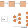
Structure of the proposed CTMF-Net

Figure 2 presents the structure of the proposed CTMF-Net. In this network, BUS images are first inputted into the CNN and transformer branches, respectively. The CNN branch uses the VGG network as its backbone, which is divided into four stages. At the end of each stage, a CBAM is utilized to calculate spatial and channel attention weight maps. These weight maps are then multiplied element-wise with the original input feature maps, which help to enhance the relevant features and suppress irrelevant features. In the transformer branch, we first converted the spatial information of the image into sequential data that the model could process sequentially, which is known as image embedding. Image embedding is obtained by reshaping the image into patches, flattening these patches into 1-D vectors, and then mapping them into a higher dimensional space through a trainable linear projection. Then, to facilitate interaction between the intermediate features of the CNN and transformer branches, the transformer branch is also divided into four stages, with each stage containing three transformer blocks.

The proposed FIM acts as a bridge for feature interaction between the two branches. It follows each stage and takes features maps from the corresponding stages of both branches as input. The features maps of the CNN branch can be directly input into the FIM, while those of the transformer branch need to perform up-sampling to match feature dimensions with the CNN branch. The FIM output serves as the input for the next stage in the CNN branch, helping it learn global relationships between different regions. After the four stages, these features are concatenated to form a 1-D feature vector that is twice the original length and is then inputted into a multi-layer perceptron (MLP) layer for classification.

Feature interaction module. Before we delve into a discussion of fusion module features, it is crucial to first clarify two foundational concepts. CNNs excel at extracting local features by focusing on small segments of input data through convolutional filters, allowing them to build a hierarchy of features. In contrast, ViTs use self-attention to assess relationships across the entire image simultaneously, enabling them to capture complex global contexts and long-range dependencies directly. Given these distinct characteristics, it is natural to think of a feature fusion strategy that uses a transformer branch with global information to guide a CNN branch with local information. This approach, which mirrors human visual perception from global to local, enhances both the efficiency and accuracy of the network.

Figure 3 shows the structure of our proposed FIM. It serves as a bridge between CNN and transformer branches, facilitating the interaction and fusion of intermediate features from both branches and guiding the CNN branch to learn global features from the transformer branch. This module effectively addresses the different features between the two branches and avoids a learning process dominated by an individual branch.

The pseudocode of the FIM is shown in [CR] . We assumed that the features input into the FIM from the CNN and transformer branches were F Conv and F Transformer , ∈ C × H × W , respectively. The FIM first projects F Conv to the value, V , and the key, K , then projects F Transformer to query, Q . In attention mechanisms, Q is used to search for information, K is used to match these queries to determine the focus of attention and V contains the actual informational content, which is selected and processed based on the matching results [ ]. The collaboration of Q , K and V enables neural networks to dynamically extract the most relevant information from large datasets. As transformers are adept at extracting global features, using the globally sensitive features they derive as Q can effectively guide integration and reshaping of local features extracted by CNNs, which are projected to V and K . We used a multi-head attention mechanism to fuse the features, which started by linearly projecting Q , K and V into multiple sets of Q , K and V . It then computed attention scores for each set through dot products, scaling and softmax operations. The scores were used to aggregate weighted sums of V . The outputs of each head were concatenated and transformed through one final linear projection to produce the output. The formula for calculating multi-head attention is as follows ( eqn [1] ):

Attention(Q,K,V)=softmax(QKTC)V

where Attention ( · ) is multi-head attention.

Algorithm 1

Feature interaction module

1:	# L : linear projection layer
2:	# L N : Layer norm
3:	# M L P : Multi-layer perceptron
4:	Input: Features from the CNN branch F c o n v and features from the transformer branch F _transformer
5:	F _tmp← F _conν;
6:	For i = 1 to 2 do
7:	Q, K, V ← L ( F _transformer), L ( F _tmp), L ( F _tmp) ;
8:	Calculate multi-head attention Attention(Q,K,V) via Eq. (1) ;
9:	Calculate F’ _Convvia Eq. (2) ;
10:	Calculate F” _Convvia Eq. (3) ;
11:	F t m p ← F” _Conv;
12:	end for
13:	F Conv mid ← F tmp ;
14:	Calculate F Conv out , the result feature map after the FIM via Eq. (4)

After calculating the multi-head attention, its output was combined with F Conv through a residual connection to form F Conv ′ , which was then fed into an MLP. The result from the MLP was again combined with F Conv ′ through a residual connection. The formula was calculated as follows ( Eqs. (2) and (3) ):

F′Conv=FConv+Attention(Q,K,V)

F″Conv=F′Conv+MLP(LN(F′Conv))

where F ′ Conv and F ″ Conv are intermediate results and LN(⋅) is Layer − norm. The above process was performed twice to obtain the interactive feature map F Conv ′ mind , and the result was output after passing through a rectified linear unit (ReLU) activation function and a convolutional layer with a 3 × 3 kernel as follows ( eqn [4] ):

FConvout=Conv(ReLU(FConv+FConvmid))

where F Conv out is the result feature map after the FIM and Conv is a simple convolutional layer.

Convolutional block attention module. Figure 4 shows the structure of CBAM, which was employed after each CNN stage to enhance relevant features and suppress irrelevant features. It comprises the channel attention module (CAM) and the spatial attention module (SAM), which respectively apply channel and spatial attention. This combination of channel and spatial attention mechanisms is generally superior to the squeeze-and-excitation module (SE) [ ], which only incorporates channel attention. Specifically, we followed Woo et al.’s design [ ] and chose the strategy that channel attention comes first, followed by spatial attention.

The CAM calculated the channel attention weight vector with three steps. First, the global max pooling and average pooling layers were applied to obtain two channel feature vectors. Second, these two channel feature vectors were fed into a shared-weight MLP network to compute the channel attention weight vectors. Finally, the two channel attention weight vectors were summed element-wise and passed through a sigmoid layer, obtaining the final channel attention weight vector. The CAM can be defined as ( eqn [5] ):

Mc(F)=sig(MLP(Avgpool(F))+MLP(Maxpool(F)))

where M _c(.) is the channel attention weight map, F is the input feature map, sig(⋅) is sigmoid function, MLP(⋅) is multi-layer perceptron, Avgpool(.) is average pooling and Maxpool(.) is max pooling.

The SAM calculated the spatial attention weight map with two steps. First, the global max pooling and average pooling layers were utilized to obtained two spatial features maps. Second, the two spatial features maps were concatenated and sent to a convolutional layer to generate the spatial attention weight map. The SAM can be defined as ( eqn [6] ):

Ms(F′)=sig(Conv([Avgpool(F′);Maxpool(F′)]))

where M _s (⋅) is the spatial attention weight map, F’ is the multiplication of the channel attention weight vector and the original feature map and Conv(⋅) is the convolutional layer with a kernel size of 7.

Implementation details

In this study, we trained the network using the PyTorch [ ] deep learning framework on a single Nvidia GTX 3090 GPU. For training purposes, we utilized an open-source pre-trained model called Vit_B_16_imagenet1k, which was initially pre-trained on the ImageNet21k dataset and fine-tuned on the ImageNet1k dataset. We also implemented early stopping, with a maximum epoch number of 100 to prevent overfitting. The Adam optimization algorithm was utilized for training with a batch size of 16, a learning rate of 1e-4, and a decay rate of 1e-1. The weighted binary cross-entropy loss function was adopted as the loss function for the BUS classification task, a binary classification problem. This choice takes into account the imbalanced distribution of samples in the dataset, allowing us to assign different weights to positive and negative classes to mitigate the effects of imbalance. The loss function can be written as ( eqn [7] ):

L=1N∑i=1N−[w·yi·log(pi)+(1−w)·(1−yi)log(1−pi)]

where N denotes the sample number, w is decided by the ratio of the positive example, y i is the ground truth of the i ^thsample and p _iis the predicted probability of the i ^thsample. To prevent overfitting, image augmentation was implemented for the training sets, which included image flipping, cropping and applying adjustments to brightness, saturation and contrast.

For training and testing, both SYSU and UDIAT datasets were randomly divided into five groups for five-fold cross-validation. The SYSU dataset contains a total of 980 images evenly split into five groups of 196 samples each, and the UDIAT dataset consists of 163 images distributed into groups of 33, 33, 33, 32 and 32 samples. For these two datasets, we conducted a total of five training sessions. In each session, four groups were used as the training set and one group as the validation set. After completing five training sessions, every group of data was validated, ensuring comprehensive utilization of the data. This cross-validation approach enabled us to train and test the model on different data sub-sets for a comprehensive evaluation of classification performance. The BUSI dataset, serving as an external validation set, includes all 647 images used for testing without any further division. To ensure consistency and comparability, all BUS images from the SYSU, UDIAT and BUSI datasets were resized to 224 × 224 pixels. Additionally, to maintain data integrity, we carefully reviewed and filtered the data to ensure that no multiple samples from the same tumor were included across the three datasets.

Evaluation metrics

In this study, we quantitatively evaluated all networks using various metrics, including accuracy, recall (sensitivity), precision, F1 score, AUC score and balanced accuracy.

Accuracy is the most intuitive indicator of the model’s classification performance, representing the proportion of correctly classified samples in all samples. Accuracy was calculated through the following Eq. (8) :

Accuracy=TP+TNTP+FP+TN+FN

Only gold members can continue reading. Log In or Register to continue