Key Points
Neurosonography of the fetus and the neonate is an informative and noninvasive as well as inexpensive modality that is of great benefit in clinical diagnosis.
As technology improves and our understanding of sonoanatomy of the fetal and neonatal brain widens, the distinction between normal and abnormal, as far as anatomy is concerned, becomes increasingly possible.
Anomalies and disease of the developing brain area are common. In order to diagnose a deviation from what is normal, it is important to understand and recognize the developmental milestones of the normal brain how it grows, and matures, reaching its almost final anatomy at birth.
This chapter presents the sonographic landmarks of developing embryonic and fetal CNS and also suggested new ways to study it systematically.
The introduction of TVS in fetal neurosonography adds an additional powerful tool to the diagnostic algorithm, increasing diagnostic precision in patients suspected of an anatomically abnormal fetal CNS.
In the future, 2D as well as 3D fetal neurosonography will be used routinely in all pregnant patients to examine the developing brain, the same way we now examine other fetal organs and organ systems.
Problems of the central nervous system (CNS) can range from very simple, that is, merely a variance of the normal, to the most devastating diseases incompatible with life. It is important to recognize these anomalies as the fetus is scanned throughout gestation, starting very early in the first trimester to late in the third.
The prerequisite for differentiating normal from abnormal structures is a thorough knowledge of the CNS anatomy. It is beyond the scope of this and the following chapters to teach the reader advanced neuroanatomy; however, special emphasis is placed on describing basic but sufficiently detailed sonographic neuroanatomy to recognize structures seen by transabdominal (TAS) or transvaginal sonography (TVS). Those interested in scanning the fetal brain to detect deviations from the norm should first refresh their knowledge of neuroanatomy.
It is not sufficient to know only the anatomy of the full-term fetal or neonatal brain. Dealing with the sonographic anatomy and pathology of the fetal brain requires an additional dimension that is of the utmost importance for correctly evaluating the CNS at various prenatal ages of the fetus, that is, knowledge of the evolution of structures from about 6 to 7 postmenstrual weeks to the time of birth. Almost all organs and organ systems are in place by the end of the embryonic period. However, only at approximately 14 to 16 postmenstrual weeks would some of them—the heart and the kidneys, for example—perform almost at the level of perfection in the final month.
All that most organs do during the fetal period is increase in size. The brain, on the other hand, undergoes major developmental changes almost until the last several postmenstrual weeks of intrauterine life. Good examples of this are the changes in the size of the ventricles; the appearance and completion of the development of the corpus callosum; and the deepening, branching, multiplying, and growth of the sulci and the gyri. It is therefore essential to understand the development of various parts of the prenatal brain in order to evaluate it and differentiate abnormal from normal development.
We deal with the prenatal brain in this book. This chapter covers normal anatomy as viewed by sonography, emphasizing the development of the fetal brain from 6 to 7 postmenstrual weeks to term. Of course, the CNS starts to develop at much earlier prenatal ages. However, at these very early prenatal ages, probably up to 7 postmenstrual weeks, the tiny structures still cannot be recognized by presently used ultrasonographic technologies. These methods were dealt with in Chapter 1, on the embryology and development of the early prenatal brain. This chapter therefore will begin with the description of the sonographic appearance of the CNS starting at 6 to 7 postmenstrual weeks.
The reader’s expectation for this chapter should be limited to enhancing his or her understanding of the normal prenatal brain anatomy before engaging in the diagnostic process and describing its pathology.
The customary ultrasound (US) equipment is used in imaging the prenatal brain. The two types of US probes employed are the transabdominal and transvaginal US transducer probes. Imaging the fetal brain depends on penetration of the sound waves as well as acoustic impedance of the tissues along the sound path. The acoustic impedances of most biologic tissues are similar. Therefore, only a small fraction of the sound is bounced back at each of these interfaces. The sound is thus successfully transmitted to deeper tissues, which can then be imaged. The soft tissue–bone interface is an exception to this rule. Bone has much higher impedance; thus, at the interface, due to the reflected sound, a very strong echo is produced. The sound energy reflected back is significant, and only a fraction of the attenuated sound waves are transmitted to deeper structures. To illustrate the magnitude of this effect, the acoustic impedance of bone is about 7 times that of water or soft tissues in the fetal body. Imaging of structures behind bone therefore becomes problematic because an acoustic shadow is created. As the fetal skull bones thicken and calcify during the course of gestation, fewer and fewer sound waves penetrate to enable imaging of the brain.
Imaging is also frequency dependent. The higher the frequency is, the better the resolution of the picture. However, the price we pay for increased picture resolution is reduced penetration, or the reduced half-intensity depth. The latter describes the ability of sound to penetrate and is expressed as the thickness of the tissues at which the sound intensity is reduced by half. This half-intensity depth decreases with increased frequency, correlates well with the attainable imaging depth, and is greatly dependent on the medium in which it travels. Excellent through transmission of sound in fluids such as blood or even in body tissue results from their weak sound-absorbing properties. However, bone and air strongly attenuate the intensity of sound. It is clear that the high acoustic impedance of the skull bone, as well as its property to attenuate the intensity of sound, greatly influences the way the brain can be imaged inside its bony case.
It was necessary to find imaginative ways to scan the fetal as well as the neonatal brain. By nature, transabdominal probes use lower frequencies to obtain deeper penetration and greater half-intensity depth. This is one way to penetrate beyond the bony skull. Another way is to scan through “windows” of the skull. These windows are, of course, the fontanelles. The younger the fetus is, the larger the fontanelles and sutures. Because these fontanelles measure ~1 to 2 cm in width, it is natural that sector or curvilinear scanners having a small footprint yield a better picture of the fetal and neonatal brain. These special transducers yield images that are of diagnostic value, even if they are acquired via the transabdominal route using the relatively open sutures, and fontanelles (Figure 2–1A).
Figure 2–1A.
Schematic and 3D ultrasound illustration of the fetal skull showing its bones, sutures, and fontanelles. The spaces between the bones can be used as access to the brain. (A) Lateral, posterior and superior views (www.uprightdoctor.files.worldpress.com), (B) and (C) are 3D maximum mode displays of cranial bones and sutures.

Another inventive way to scan the fetal brain is to use extremely high-frequency probes, such as 6.5 to 7.5 or even 9 MHz. Such probes are used in transvaginal gynecologic scanning. If the fetus is in the vertex presentation, it is relatively easy to maneuver the fetal head and the vaginal transducer into a position from which the device can “see” through a fontanelle. If this is successfully achieved, extremely clear pictures of the fetal brain from 13 postmenstrual weeks to term can be obtained.
Since we became aware of the possibility of obtaining limited access to the brain using the transvaginal probe, we have been using it whenever possible (ie, when the fetus is in the vertex presentation). The rather narrow but still open “window” or space between the two parietal bones; namely, the sagittal suture enables by placing the footprint of the vaginal probe over the sagittal suture, a satisfactory picture of the mid-brain structures in the median plane can be obtained. Because of the narrow nature of this space, it is almost impossible to obtain an image of lateral structures.
Transabdominal scanning of the fetal brain using the anterolateral fontanelle or the squamosal suture can, in certain cases, yield clear and clinically diagnostic images. However, the younger the fetus is, or the smaller the structure in question is that must be scrutinized, the more the transabdominal probes will be at handicap as opposed to the higher-resolution transvaginal probes. Under matched conditions the transvaginal probes, which operate at higher frequency, produce better and clinically more useful pictures.1
Lately, electronically steered transducers can improve image quality obtained by the abdominal route. This modality employs compound scanning techniques.
Over the last several years, three-dimensional (3D) has become more readily available; therefore, a short explanation of these probes and their use is in place. Both the transabdominal and the transvaginal 3D US probes (at this time) are mechanical transducers. They are controlled by a timing module that determines the number of continuously advancing US pictures acquired and saved into a volume. The acquisition speed ultimately determines the picture resolution and quality. For moving structures (eg, a moving fetal part), high acquisition speed is required; for stationary organs (eg, in gynecology), lower acquisition speed is adequate, which enables obtaining many more sections, hence a higher-resolution end product. In view of the fact that the fetal brain is a stationary organ (except when the fetal head moves), when scanning the fetal brain, one can select a lower acquisition speed. The technique of 3D volume acquisition is relatively simple, and given that an increasing number of new US machines offer 3D technology, it is essential that those readers interested in enhancing their fetal neurosonography skills get acquainted with this powerful scanning technique.
Fetal brain scanning has emerged from the vast experience gained with neurosonographic imaging of the neonate. The fetal as well as the neonatal head is scanned using the three main body coordinates: the sagittal, coronal (frontal), and horizontal axial planes (Figure 2–1B). Initially, scanning of the neonatal brain was done through the temporal region, obtaining axial sections.2,3,4,5,6,7,8,9 To achieve this imaging, lower-frequency transducers were used. Two factors contributed significantly to the improved resolution of one neonatal scan: the higher-frequency US transducers (mainly the sector and the small-footprint curvilinear probes) and use of the anterior fontanelle as an acoustic window. The pictures obtained are in the median, paramedian, and different coronal sections, as well as oblique, sections.10,11,12,13,14,15,16,17,18,19 It should be stated at the outset that TAS of the fetal brain usually provides axial and coronal sections. However, it is extremely difficult or almost impossible to obtain sagittal sections (Figure 2–2). At times, though, sagittal sections are needed for imaging of different pathognomonic features and diseases of the brain. Transvaginal scanning through the anterior fontanelle provides us with such median, paramedian, coronal, and oblique sections, much like neonatal scanning (Figure 2–3).20 Another advantage of scanning the fetal brain using TVS is that the scanning planes obtained are identical and therefore comparable to those performed in the neonate. Continuity of follow-up and comparison between fetal and neonatal scans are then possible by pediatric neurologists and neurosurgeons. The input of these consultants is therefore relevant even in the prenatal period.
Figure 2–1B.
The “classical” planes used in the imaging of the fetal brain. The vertical planes are either coronal or sagittal. One of the latter planes is the median plane. There are infinite numbers of coronal and sagittal (paramedian) planes. As far as fetal neurosonography is concerned, the coronal and sagittal planes are reached through the anterior fontanelle in a fetus presenting with the vertex. Several sections through each plane can be generated. The horizontal (axial) planes are achieved classically by a transabdominal 3D scanning.


Figure 2–3.
Schematic drawing depicting the technique of transvaginal sonography during the second and third trimesters. Inset: The relationship of the anterior fontanelle to the transvaginal transducer is demonstrated. (From Monteagudo and colleagues, 1991,20 with permission.)

An issue of some importance is that fetal neuroimaging requires the use of an end-firing, symmetrical, in-axis (or in-line) vaginal probe. Using an end-firing, off-axis vaginal probe makes symmetrical imaging of the brain and maneuvering of the probe extremely cumbersome (Figure 2–4). The orientation process is also affected, with regard to its speed, simplicity, and teaching. Most off-axis probes require constant use of the left-right orientation key on the control panel to correctly display orientation on the picture.
Figure 2–4.
The different scanning planes of the transvaginal probes most often used. (A) Transvaginal fetal neuroscans are imaged best with an end-firing, symmetrical, in-axis probe. (B) The tilted, off-axis scanning plane generated by a curvilinear transvaginal probe. In order to scan hemispheres at the same time, the shaft of the probe must be moved from side to side. This may be uncomfortable for the patient, or it may simply be impossible. At times, the probe must be rotated 180° to direct the scanning plane to the other hemisphere.

Blaas et al21 described the use of the 3D US probe. The development of the three different structures in the brain was defined using this technique. The information obtained by this “spatial scan” was stored in the computer and enabled the user to obtain different pictures, creating not only coronal, sagittal, and axial planes but also selected planes to highlight the spatial embryonic brain anatomy (Figure 2–5) and pathology. Until the 3D technology becomes universally available and widely used, we must mentally re-create the necessary planes and sections. Thus, knowledge of neuroanatomy remains an important issue.
Figure 2–5.
In vivo 3D ultrasound reconstructions of embryos and early fetuses. (From Blaas HG, 1998,21 with permission.)

Another technique that can be used to better describe the anatomy of the fetal brain is color Doppler flow studies. If color flow studies are used, a textbook on neuroanatomy, particularly on the arterial and venous network of the fetal brain, should initially be studied. Color and power Doppler flow studies may become important when anatomical structures such as space-occupying lesions, degenerative changes, or hemorrhages of the brain are examined. Another area still under investigation is the physiology of the blood supply to the brain. This is covered in Chapter 15.
Because TAS is easy to perform and is used routinely by those who engage in ultrasonography of the fetus, it seems redundant to describe its technique. Transvaginal two-dimensional (2D) and 3D scanning of the fetal brain, however, requires more experience and is skill dependent; therefore, we describe it here in detail.
Obviously, due to its small size, the embryonic and early fetal CNS requires the use of a high-resolution transvaginal US probe.22,23,24,25,26,27,28,29,30 The CNS structures seen in the first trimester are described later.
Scanning the fetal brain in the second and third trimesters via the vaginal route requires the same safety guidelines used for the customary speculum and palpatory examinations during pregnancy. If these can be performed safely in the second trimester, there is no contraindication to insertion of the vaginal probe for scanning the fetal brain. Of course, as stated before, the fetus must be in the cephalic presentation. At times, when it is of the utmost importance to obtain accurate and more detailed information regarding a disease state, or if an additional sagittal view would significantly contribute to the diagnostic process, it may be important to consider the external cephalic version of the fetus. When a second-trimester fetus is scanned, such a change in the fetal presenting part most of the time can be brought about without effort or can occur spontaneously.
Transvaginal 2D and 3D neuroscanning can be used as early as 10 to 14 postmenstrual weeks. Its technique is relatively simple.21,24,31,32 The transvaginal probe is prepared in the customary fashion, covering it with a clean condom or one of the digits of a surgical rubber glove after contact gel has been applied to the tip of the probe and, finally, applying some lubricating (K-Y) gel onto the covered tip, making it ready for vaginal insertion. Due to increasing reports of latex allergies in the population, special prelubricated polyvinyl vaginal probe covers are available. The patient should be in the lithotomy position, preferably lying on a gynecologic examination table. Constantly following the image created by the advancing probe on the monitor, the first structure to be viewed (and evaluated as well as measured) is the cervix. The tip of the probe is typically placed on top of the anterior cervical lip. If the patient’s bladder is full and displaces the fetal head upward, the patient should be asked to void before the examination proceeds.
To obtain a clear image of the fetal brain, it may be necessary to maneuver the probe and/or the fetal head into the most convenient position. This will be achieved if the axis of the probe and the median plane of the fetal brain (ie, the falx cerebri) are in line (Figure 2–3). Usually, the operator must use both hands to point the probe to the anterior fontanelle or along the metopic and/or sagittal sutures and hold the fetal head in the desired position. Unless skilled help is available to freeze the image and trigger the recording device, a foot pedal is necessary to perform all of the necessary tasks at the same time. An active fetus may be extremely hard to stabilize by the abdominally placed second hand of the operator. To wait for the fetus to enter a quiet sleep state (state IF) may be a time-consuming option. However, the scanning of an almost motionless fetus in deep sleep does have its dividends.
In addition to the previously mentioned advantages and disadvantages of TAS and TVS of the fetal CNS, another caveat should be introduced. At times, it is hard or too time-consuming to obtain perfect planes and classical sections of the brain using TVS. This is, of course, a result of the somewhat limited mobility of the vaginal probe and/or the almost constantly moving fetus. Sometimes the fetal head position is such that it prevents the imaging of clear planes. Complementing the scan with an attempt at TAS, rescheduling the scan, or simply allowing the patient to walk for some time may improve the results.
Figure 2–1B depicts the three well-known classical planes of the body, in terms of its planes and sections. These are described below. Additional terms used in the orientation process are rostral or anterior (toward the face); occipital, posterior, or nuchal (toward the back); left lateral or right temporal (toward the respective ear); caudal, basal, or inferior (toward the base of the skull); and medial (toward the middle). It should be noted that the sagittal plane traversing the middle of the body is termed the median (do not use “midsagittal”) plane (see Chapter 1).
Ultrasonographic images of the embryonic (up to 9 postmenstrual weeks) or fetal (at and after 9 postmenstrual weeks) period is heavily dependent on several factors. The first factor is the resolution, which, in turn, is a function of the frequency at which the crystals operate. The frequency and, in some ways, the diameter of the piezoelectric crystal determine the slice thickness. The thicker the slice that is insonated and imaged, the more information is “collapsed” into the 2D picture seen on the screen. This slice thickness may, in many cases, be several millimeters. In the case of an embryonic brain at 7 or 8 postmenstrual weeks, the median imaging plane may include the entire width of the head due to the relatively thick imaging slice (Figure 2–6A). This is true even for a high-frequency transvaginal transducer; in the axial or coronal planes, it may be possible to obtain several sections due to the somewhat larger size of the growing embryo (Figure 2–6B and C).
Figure 2–6.
The effect of slice thickness, or the third dimension of ultrasound imaging, is demonstrated. (A) Due to the slice thickness, even at the focal point, a scan in the median plane may include the entire width of the embryonic head. (B), (C) In axial or coronal planes, two or three sections may be possible. Starting with the fetal period, an increasing number of sections become feasible.

Controlling the thickness of the slice becomes important in postprocessing of 3D US pictures derived from the volume scan. Using the software of several 3D US machines, it is possible to select the desired slice thickness, thus enhancing the displayed image clarity.
Around 9 postmenstrual weeks the size of the embryonic head becomes large enough to yield several sections in each of the three cardinal planes. Because of the small head size, the sections can be obtained in almost a perfect parallel fashion. This becomes increasingly difficult later in pregnancy, as discussed in subsequent sections.
It should also be clear that the terms axial (horizontal) and coronal (frontal) planes refer to the trunk and become somewhat unclear if applied to the anteflexed embryonic head. Therefore, a coronal plane of the trunk would be axial of the flexed head. It is our understanding, therefore, that the term axial in an embryo at 8 to 10 postmenstrual weeks is in a plane parallel with the base of the skull or the orbitomeatal plane (see Chapter 1). A coronal plane of the same fetus is one at 90° to the axial plane (Figure 2–7).
Figure 2–7.
Due to the flexed posture of the embryonic or early fetal head, the plane that is coronal as far as the trunk is concerned becomes an axial plane when applied to the brain. In the same way, if an axial or transverse section of the trunk is applied to the head, it generates a coronal section of the brain.

If for any reason (eg, research or clinical observation) it is necessary to image the brain in the first trimester, the observer should place the region of interest rigorously into the exact focal point of the transducer. Thus, it is essential to be knowledgeable about the respective transducer specifications in order to generate high-quality images.
With its increasing size, the developing fetal brain becomes progressively available for high-frequency 5 to 12 MHz TVS. The pictures obtained in the different scanning planes are thus of diagnostic quality. In other words, major diseases of the CNS can be diagnosed, starting at 9 to 11 postmenstrual weeks.
With regard to scanning the fetal brain after 12 weeks, especially after weeks 14 to 15, it is at this point that the thickening skull bones attenuate the high-frequency sound waves of the vaginal probe to a very low level, making imaging from any randomly selected direction increasingly impossible. This is the time at which the window to the fetal brain (ie, the fontanelle) becomes important. This relatively narrow gateway for the sound waves forces certain restrictions on the sonologist or sonographer. First, the tip of the transducer must be kept over the fontanelles or the sagittal (or metopic) suture, to achieve the full scanning potential of the sound output. Second, the different scanning sections in the sagittal, coronal, and oblique planes should be generated by tilting the transducer back and forth (Figure 2–8). Because of the reasons mentioned, these successive sections are not parallel to each other in any given plane, as, for example, with the shifting but always parallel planes of computed tomography (CT) and magnetic resonance imaging (MRI).
Figure 2–8.
Scan through the anterior fontanelle. (A) The limited motion of the probe within the vagina allows the median plane to be visualized, whereas on each side of it, the planes are oblique and not parallel, and therefore cannot be regarded as strictly sagittal. (B) Similarly, a coronal plane can be obtained, whereas those in front of and behind it are oblique planes, not subsequent coronal planes. (C) The horizontal planes can be achieved using the transabdominal approach.

This transfontanelle scanning by TVS, common to prenatal and neonatal brain scanning, is really performed in a “radial” fashion. Some of the sagittal and coronal sections are therefore oblique-sagittal and oblique-coronal sections. In the sagittal plane, then, left and right oblique sections are generated; in the coronal plane, occipital and frontal oblique sections are generated (Figure 2–8).
However, as we will see later, if a 3D brain volume is acquired, regardless of the transducer or the scanning route used, the final display will use perfectly parallel planes and sections, as in MRI and CT.
It is important to understand that in order to scan the fetus presenting with the vertex, the free motion of the vaginal probe is restricted by the anatomical limits of the vagina. Only a few “classical” or “pure” planes can therefore be achieved: the median and one coronal plane. In the sagittal planes (to use the best approximation), because of the fan-shaped, radial scanning sections, several left and right oblique sections can be generated on each side of the median plane (Figure 2–8). This is partially overcome by using 3D US. In front of or behind the coronal plane (once again, to use the best approximation), several frontal and occipital oblique sections can be generated (Figure 2–8).
If several sections are created, the 3D anatomy should be re-created mentally by the observer. This “mental processing” will be less and less necessary by the introduction of 3D multiplanar imaging. Three-dimensional imaging of the fetal brain will also eliminate the “radiating” planes, as all planes will be parallel with each other.
If the second- or third-trimester fetus assumes an asynclitic head position, it is sometimes possible to obtain axial planes. The same is true if the head assumes a flexed occipitoanterior position. A detailed study of the posterior fossa should be performed as soon as this presentation is detected. After some time, due to fetal movement, this presenting anatomy may shift away, not to return for the duration of the examination.
As the examination proceeds, we have observed certain conventions in orientation. This serves to introduce a systematic way of displaying the images.
In the sagittal planes the fetal face or the frontal direction should be almost uniformly oriented to the left of the picture. This will orient the posterior fossa and the occipital structures toward the right side of the screen. Likewise, if the lateral ventricles are imaged using these planes, the anterior horn should point toward the left and the posterior horn toward the right side of the monitor.
In the coronal planes the pictures should be taken in such a manner that the fetus should face, or look right at, the examiner. This means that by convention—as is customary in imaging laboratories—the right side of the brain will appear on the left side of the screen, whereas the left side of the prenatal brain will point toward the right of the picture. If no annotation is to be seen on a hard copy, it is assumed that the above-described orientations of the prenatal brain sections in the coronal planes were observed. It seems best, however, to indicate the orientation of the left or right side on at least one of the images. This annotation of the left or right side becomes crucial if an asymmetrical or unilateral lesion is detected.
If 3D US is used, one should be acquainted with the initial display of the orthogonal planes inherent to the different manufacturers’ systems. These orthogonal planes are the customary initial planes appearing on the screen after the acquisition of the volume is completed. Determining the correct side is essential when unilateral brain pathology is encountered.
This section deals with the sonoembryology and sonoanatomy of the prenatal brain as it appears and as a continuous function of structural development. It should be clear that parts of the prenatal brain exist and are in different developmental stages even before they can be imaged by ultrasonography. This is particularly true for brain structures revealed by a scan performed during the first 12 to 14 postmenstrual weeks of pregnancy. The structure may well be in place, but due to its size and location, the angle of insonation may not be obvious to the observer. Other structures develop later as a normal process, and because of this they are not seen on early scans.
We present here the normal embryonic and fetal neurosonology in two sections. The first subsection deals with the period up to 9 postmenstrual weeks. The second section comprises the weeks following the ninth postmenstrual week. This is an entirely arbitrary partition. Starting from the 13th postmenstrual week, some of the structures imaged by high-frequency transvaginal transducers are of clinically usable quality. This is also the time after which multiple and clearly discernible brain sections can be obtained using the standard planes.23
To better understand the development of the embryonic brain, the reader is referred to Chapter 1. After reading that chapter, a clearer perception of the sonographically visualized structures will be possible.
As concerns the age of the embryos and fetuses, the arguments and debates are well known and well documented. Chapter 1 provides the tools to understand the different views. Table 2–1 contains the embryonic and fetal age conversions, which will allow quick reference for those who would like to rely on the date of the last menstrual period (LMP) to calculate age, as well as for those who are used to expressing age in terms of weeks or days from fertilization (if such a date is known).33 O’Rahilly and Müller34 indicated that points C and R of the crown-rump length (CRL, Figure 2–9) are imprecise and frequently are difficult to determine. They emphasized that the best single measurement is the greatest length (GL), exclusive of the lower limbs, and its determination is practicable in both the embryonic and fetal periods. Subsequently, Goldstein35 expressed concern about measuring the longest diameter of the developing embryo sonographically, calling it the CRL. His measurement, according to the study, does not follow the curvature of the curled-up embryonic body. Therefore, it actually measures the longest diameter (ie, the GL of O’Rahilly and Müller34) or the size of the embryo. Goldstein35 proposed the term early embryonic size (EES) for the sonographic measurement. Table 2–1 also contains the EES measurements and their conversions to embryonic age.
| Postmenstrual Week | Time From LMP (Weeks and Days) | Time From Fertilization (Weeks and Days) | Days From Fertilization | Crown–Rump Length (cm)a | EES (mm) |
|---|---|---|---|---|---|
| 7th | 6 + 0 to 6 + 6 | 4 + 0 to 4 + 6 | ~28–34 | 0.42–0.81 | 1–6 |
| 8th | 7 + 0 to 7 + 6 | 5 + 0 to 5 + 6 | ~35–41 | 0.89–1.38 | 7–13 |
| 9th | 8 + 0 to 8 + 6 | 6 + 0 to 6 + 6 | ~42–48 | 1.47–2.08 | 14–20 |
| 10th | 9 + 0 to 9 + 6 | 7 + 0 to 7 + 6 | ~49–55 | 2.19–2.92 | b |
| 11th | 10 + 0 to 10 + 6 | 8 + 0 to 8 + 6 | ~56–62 | 3.05–3.89 | b |
| 12th | 11 + 0 to 11 + 6 | 9 + 0 to 9 + 6 | ~63–69 | 4.04–5.00 | b |
| 13th | 12 + 0 to 12 + 6 | 10 + 0 to 10 + 6 | ~70–76 | 5.17–6.25 | b |
| 14th | 13 + 0 to 13 + 6 | 11 + 0 to 11 + 6 | ~77–83 | 6.43–7.63 | b |
Figure 2–9.
The outlines of four embryos (right lateral views) with the brain superimposed. The embryos are shown at stages 13, 15, 17, and 20, respectively, and are at 6w1d, 6w5d, 7w5d, 9w1d postmenstrual weeks. In the first three examples, the greatest length (GL) is larger than the crown-rump (C–R) length, whereas the two measurements coincide in the fourth. The last drawing (stages 13 to 23) is a scheme to summarize the “ascent” of point C until the C–R length comes to equal the GL. (From O’Rahilly and Müller, 1984,34 with permission.)

Returning to the work of O’Rahilly and Müller,34 it is clear that the C point (the crown), which, in stages 13 to 20 (6w0d-9w1d from the LMP), is at the point where an imaginary line drawn along the mesencephalic flexure would touch the surface of the embryo, just above the middle of the midbrain (see Figure 2–9), is hard to find sonographically. Even if it can be determined, the CRL would yield a smaller length than the GL or the EES of Goldstein.35 Figure 2–9 depicts how the C point changes location throughout development from stage 13 to stage 20. Only at stage 23 (10w1d postmenstrual weeks) do the CRL and GL (or EES) become identical as clinically used measurements.
Using currently available US machines, the earliest scan to depict any brain structure can be performed at 7 postmenstrual weeks (5 weeks, or 35 days, from fertilization). At this age one or several sonolucent areas can be detected in the rostral and cephalic pole of the embryo. The detail of the image depends on the resolution of the equipment used.
If attempts are made to image details of the CNS before this embryonic age, a clear fetal pole, at times adjacent to the yolk sac, can be seen (Figures 2–10, 2–11 and 2–12A and B).36 However, sagittal as well as coronal sections do not yield distinct structures. At times, a tiny sonolucency is seen in the rostral part of the embryo. The nature of this structure is unknown. The parallel lines of the somites (from which the vertebrae are derived) are discernible at or slightly before 7 postmenstrual weeks (Figures 2–12C).


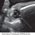
Figure 2–12.
An embryo at 7 weeks and 2 days (postmenopausal). The CRL is 12 to 13 mm. By the Carnegie classification, this corresponds to a stage 16 embryo at 37th day postfertilization. The arrows point to the rhombencephalon. (A) Sagittal image. (B) Sagittal image highlighting the heart and umbilical flow. (The patient was scheduled for a termination of the pregnancy.) (C) The parallel lines of the spinal structures are evident (ys = yolk sac).

Blaas and colleagues29,30 studied the brain structures, starting with an embryo with a CRL of 12 mm (7 weeks, 3 days from the LMP). They described the possibility of imaging the cerebral hemispheres (telencephalic vesicles), rhombencephalon, and diencephalons (Figure 2–13). In embryos with a CRL of 16 mm (8 weeks from the LMP), these structures become better defined. Thus, the interventricular foramina (Monro) can be seen (Figure 2–14).
Figure 2–13.
Transverse/oblique section through the rhombencephalon (4), diencephalon (3), and cerebral hemispheres (H) of an embryo (crown-rump length of 12 mm at 7 postmenstrual weeks 3 days). The bilateral evaginations of the hemispheres are clearly seen. There is still a wide opening to the third ventricle. (From Blaas and colleagues, 1994,29 with permission.)

Figure 2–14.
Transverse/oblique section through the rhombencephalon (4), diencephalon (3), and cerebral hemispheres (H) of an embryo (crown-rump length of 16 mm at 8 postmenstrual weeks 0 days). The borders between the cerebral hemisphere and the third ventricle (3) remain relatively small and start to develop into the interventricular foramina. (From Blaas and colleagues, 1994,29 with permission.)

Our group has scanned well-dated embryos from 7 to 10 weeks from the LMP and evaluated the structures imaged. A 6.12 MHz mechanical 3D transvaginal transducer was used. At 8 weeks, 1 day (from the LMP) in the sagittal and axial/coronal planes, we could see all the primitive ventricular suctum (Figure 2–15A, B, and C). Figure 1–4 in Chapter 1 represents a sagittal section of the embryonic brain at a comparable age.
Figure 2–15.
An 8 weeks and 1 day (postmenopausal) embryo with the crown-rump length of 16.9 mm. By the Carnegie classification, this corresponds to a stage 18 embryo at 43 days postfertilization. (A) Median picture showing parts of the anechoic ventricular system. (B) The orthogonal planes; the median axial and coronal planes. The lower limb buds and the telencephalic vesicles are highlighted by the arrows. (C) Tomographic, consecutive sagittal sections along the lines shown in the upper left image square. The picture with the white frame is the median plane of the embryo.


At 8 weeks, 1 day and 8 weeks, 3 days from the LMP (Figure 2–15), the structures appear clearer, and flexures of the brain, such as the mesencephalic and pontine flexures, were located. The coronal sections revealed the rhombencephalon with regard to the major divisions. Figure 1–4 in Chapter 1 depicts a median section of the brain at 8 weeks, 3 days after the LMP. The subdivisions of the brain (Figure 2–16) could not yet be sufficiently discerned by TVS.37
Figure 2–16.
The divisions, subdivisions, and brain cavities seen in an infant’s brain. The metencephalon consists of the cerebellum and the pons. The myelencephalon is the medulla oblongata. The brain stem comprises the midbrain, pons, and medulla. The third ventricle is mainly diencephalic, but it is partly telencephalic. The central canal is mainly in the spinal cord, but it is partly in the medulla. All of these parts are present by 5 postfertilizational (7 postmenstrual) weeks. The subdivisions and the cavities can be detected by high-frequency transvaginal sonography, but only from about 8 to 8½ postmenstrual weeks. (From O’Rahilly and Müller, 2001,37 with permission.)

At 8 weeks, 5 days from the LMP (Figure 2–17), the embryo starts to “unfold.”23 The mesencephalic flexure is almost in line with the longitudinal body axis. The cavities of the ventricular system are clearly identifiable. Subdivisions such as the telencephalon, diencephalons, metencephalon, and myelencephalon are seen sonographically not only on sagittal but also on coronal sections.
Figure 2–17.
Median and coronal (posterior oblique) sections of an embryo at 8 postmenstrual weeks and 5 days (crown-rump length, 20 mm). (A) Median section showing the following structures: telencephalon (Te), diencephalon (Di), and mesencephalon (Mes). The metencephalon (Met) and myelencephalon (My) are parts of the rhombencephalon (R). The two main flexures, pontine (PF) and mesencephalic (CF), are also seen. (B) Coronal oblique section through line b. (Modified from Timor-Tritsch and colleagues, 1991,23 with permission.)

In addition to the already described structures, the choroids fold and slightly later, at 8 weeks, 5 days from LMP, the first sighting of the choroid plexus was reported. Only days later, at 9 weeks, 3 days from the LMP (with a CRL of 25 mm), a better image of the choroid plexus and the cerebellum was seen (Figure 2–18).
Figure 2–18.
Coronal section at 9 postmenstrual weeks and 3 days, showing the rhombencephalon (crown-rump length, 25 mm). The mesencephalon, cerebellum, and choroid plexus are marked. (Courtesy of Blaas, Department of Obstetrics and Gynecology, National Center for Fetal Medicine, Trondheim University Hospital, Trondheim, Norway.)

From about 9 weeks from the LMP, there is a significant change in the TVS evaluation of the fetus as a whole, particularly of the CNS. Because of their gradual development and increase in size, more structures are better seen. The development of the tortuous, fluid-filled ventricular system is readily imaged in the median plane (Figure 2–19). The subdivisions, as well as the serially connected cavities, appear on both the sagittal and coronal planes. Suddenly, it seems that many more sections can be generated in almost each of the three cardinal planes (Figure 2–19A).23
Figure 2–19.
(A) At 9 postmenstrual weeks and 1 day, it is possible to acquire multiple sections in the clanical planes. This picture illustrates five coronal sections obtained using a high frequency transvaginal probe at this age. (B) Median section at 9 postmenstrual weeks and 5 days (crown-rump length, 28 mm). The sonolucent and progressively tortuous ventricular system is imaged. Di, diencephalon; Mes, mesencephalon; Met, metencephalon; My, myelencephalon; S, the entrance to the central canal; CF, mesencephalic flexure; PF, pontine flexure. (Modified from Timor-Tritsch and colleagues, 1991,23 with permission.)

The different parts of the ventricular system are visible at this time. A study of the median section of the embryo at 9 weeks, 5 days from the LMP is depicted in Figure 2–19B. The sonolucent chain of the ventricular system winds itself around the two most prominent solid structures: the echogenic pontine flexure and the mesencephalic flexure. This age marks the stage (Carnegie stage 23) at which the latter points at the “crown” of the head and the true CRL can be measured reliably.34,35 The first rostral sonolucent structure on this image is the diencephalon. Following the diencephalon, in the caudal direction, are the mesencephalon, the metencephalon, the myelencephalon, and the part of the medulla that contains the central canal. On a paramedian section, the relatively large choroid plexus in the lateral ventricle is depicted. At this age the choroid plexus fills the entire lateral (telencephalic) ventricle. On coronal and axial sections, the falx is seen as an echogenic structure. If the choroid plexus and the falx are imaged by TVS, the age of the embryo must be at least 9 postmenstrual weeks. A reasonably high-quality, high-frequency vaginal probe is necessary to detect the falx, the different ventricles, and the choroid plexuses at or around 9 to 9½ postmenstrual weeks.
The development of the embryonic brain was previously described. As detailed in Chapter 1, the embryonic period lasts up to 8 weeks from fertilization, or roughly 10 postmenstrual weeks. Following this, the fetal period starts; this lasts until delivery takes place. From a sonographic standpoint, there is definitely no visible quantitative reason for this qualitative change. An increasing number of detectable structures are seen from 8 postmenstrual weeks on, without any significant increase at or around the cutoff age at which the designation changes from embryo to fetus.
From 10 postmenstrual weeks on, three axial, three sagittal, and three or four coronal sections in each of the cardinal planes of the fetal head can be obtained.31
A 3D model created by computer and based on serial 2D slice scans of fetuses at 8 to 10 postmenstrual weeks is depicted in Figure 2–20. The Norwegian group from Trondheim produced such computer-generated “casts” of the well-delineated ventricular system, which enabled a close study of this system as it changed shape between 8 and 12 postmenstrual weeks.38 Until a US system becomes widely available to re-create the different brain structures in a 3D fashion, we will have to rely on our own mental re-creation of fetal structures in general, and the brain in particular. To perform such a complex task in our own brain, serial sections of the structure in question must be generated and examined during every scanning session. A similar series of horizontal (axial) slices is depicted in Figure 2–21. From these images it is obvious that the choroid plexus of the fetus at 11 to 11½ postmenstrual weeks almost fills the available space within the lateral ventricle. If the gain control is increased, the high brightness of the choroid enables the detection of cysts as small as 2 to 3 mm, should they exist. The falx is sufficiently echoreflective and therefore easily seen. In addition, the third ventricle, the tentorium, the posterior fossa, and the cerebellum and its peduncles leading to the midbrain can be imaged (Figures 2–21 and 2–22). On a very low axial section the foramen magnum can also be seen (Figure 2–21C).
Figure 2–20.
Three-dimensional representation of the embryonic and fetal ventricular systems. (A) Lateral view of the brain cavities in an embryo of 13-mm crown-rump length (CRL). The outline shows the embryonic shape, with head and the umbilical cord. (B) Lateral view of the brain cavities in an embryo of 24-mm CRL. The outline shows the embryonic head and eye. (C) Lateral view of the brain cavities in a fetus of 40-mm CRL. The outline shows the fetal head and eye. (D) Oblique view of the brain cavities in a fetus of 40-mm CRL. H, cerebral hemisphere; D, diencephalon; M, mesencephalon; R, rhombencephalon; IR, isthmus rhombencephali. (From Blaas and colleagues, 1995,38 with permission.)

Figure 2–21.
Serial horizontal (axial) sections at 11 postmenstrual weeks 3 days, from the top (far left) to the base of the skull (far right). The third ventricle (3V) and the foramen magnum (FM) are seen. CP, choroid plexus; fx, falx. (Modified from Timor-Tritsch and colleagues, 1991,36 with permission.)

Figure 2–22.
Horizontal (axial) section through the head of a fetus at 11 postmenstrual weeks and 6 days (crown-rump length, 49 mm). The view is of the diencephalon (bold arrows) and its narrow third ventricle (3), and through the mesencephalon (large open arrows; M), with its wie cavity (small open arrows). AH, anterior horns. (From Blaas and colleagues, 1984,29 with permission.)

It seems that the presence of the third ventricle can clearly be seen on axial scans at 11, 12, and even 13 postmenstrual weeks (Figures 2–21, 2–22, and 2–23). However, on serial scans at 14 and 16 postmenstrual weeks (Figure 2–30), the space is progressively taken up by the expanding thalamus.
Figure 2–23.
At 12 postmenstrual weeks 1 day, a frontal oblique section (A) shows the falx and the choroid plexus. Axial sections (B, C) reveal the hyperechoic choroid plexus (cp) on top of the thalamus (T) in the lateral ventricles. Only a thin cerebral cortex mantle is still seen between the small arrows. The third ventricle (3v), the falx (f), and the frontal part of the sagittal sinus (SS) are also seen. (Modified from Timor-Tritsch and colleagues, 1991,23 with permission.)

Figure 2–24.
Serial brain sections at 14 postmenstrual weeks. 1A, 1B. Frontal oblique sections, showing the longitudinal fissure (lH) and the anterior horns (AH). Somewhat more posteriorly (1B), the choroid plexus appears (C). In sections 2 through 4 (midcoronal sections) the changing relationship of the choroid plexus (C) to the thalamus (T) can be seen. 5A and 5B are more posterior occipital oblique sections showing the cisterna magna (CM) and a bicerebellar diameter measurement of the cerebellum. (From Timor-Tritsch and Monteagudo 1991,24 with permission.)

Figure 2–25.
Serial scans of the fetal brain at 16 postmenstrual weeks. (A) An extreme anterior frontal–1 section (see Table 2–2) almost tangential to the fetal skull, showing the wide opening of the anterior fontanelle) (open arrow). (B) Frontal–2 section. The cortex and the white matter around the anterior horns are becoming progressively thicker. The sonolucency of the anterior horn (AH) is outstanding. The subarachnoid space is marked by the white arrow. (C) Midcoronal section. The choroid plexus (CP) and its connection through the interventricular foramina (small white arrows) are shown. The midline arrow indicates the falx. (D) Midcoronal–3 section through the antrum of the lateral ventricles, which are filled entirely by the choroid plexus (CP). The arrow indicates the falx. (E) Occipital–1 section. The posterior horns are marked by the small white arrows. The tentorium (t) is also indicated. (F) Horizontal section. The sonolucent cisterna magna is highlighted by the large white arrow. The cerebellum (C) and the fourth ventricle (small white arrow) are shown. The anterior horns (F) and the inferior horns (T) are visible using this section. (G) An oblique section highlighting the choroid plexus (C) and one of the cerebellar hemispheres (C) (H) Right oblique–1 section with the anterior horn (F), posterior horn (O), and choroid plexus (C) situated above the thalamus (T). The thick mass of the brain tissue is indicated by the two small arrows.

Figure 2–26.
These series of horizontal and sagittal sections are part of the workup of the posterior fossa in a normal fetus at 16 postmenstrual weeks. (A) “Low” horizontal section. The cerebellum (C) measures 1.78 cm, and the cisterna magna measures 0.66 cm. Note the inferior pedunculi (P), the hyperechoic lower portion of the vermis (V), and the fourth ventricle (small arrow). (B) The somewhat higher horizontal section of the posterior fossa, highlighting the small, threadlike structures of the arachnoid membrane (small arrows). (C) This is a higher, composite horizontal/coronal section that shows the tentorium (small arrows). The cerebellum (C) and the choroid plexus (C), and the choroid plexus (C) with a tiny choroid plexus cyst (small white arrow). (D) Almost median section showing the midbrain (MB), medulla oblongata (MO), hyperechoic vermis (small single arrow), and cerebellum (C). The tiny arrow points toward the medulla. This section clearly shows the upper portion of the medulla (multiple small arrows). (E) Paramedian section. The structures are similar to those indicated in D. (F) Median section of the suboccipital region, highlighting the cerebellum (C), cisterna magna (CM), medulla oblongata (MO), and spinal cord (small arrows).

Figure 2–27.
Additional views of the same fetus imaged in Figure 2–25. In addition, all of these images highlight the subarachnoid space. (A) Frontal–2. (B) Midcoronal–1 section. (C) Midcoronal–2 section. (D) Left oblique–1 section. The subarachnoid space is highlighted by small white arrows in all of these sections. AH, Anterior horn; F, falx; CC, corpus callosum; FM, interventricular foramina; CP, Choroid plexus; T, thalamus; OH, posterior horn. The two measurements in C are the distance from the midline to the tip of the anterior horn (1) and the depth of the anterior horn (2). These are normal for this age.

Figure 2–28.
Structural evaluation of the fetal brain at 15 postmenstrual weeks. Systematic scanning of the lateral ventricles and the choroid plexus can be performed using several horizontal or oblique planes. (A) Frontal view of the inversion rendered ventricles. (B) Lateral view of the inversion rendered ventricles. (C) Superior view of the inversion rendered ventricles. (From Timor-Tritsch and colleagues, 1995,42 with permission.)

Figure 2–29.
Composite picture of the 3D inversion renderings of the developing ventricular system from 7 to 12 postmenstrual weeks showing the lateral, frontal, and the superior views. Note the changing relations of size between the anterior horns and the rhombencephilon (fourth ventricle). (From Timor-Tritsch IE et al, 2008,39 by permission.)

Figure 2–30.
Inversion rendering of brain ventricles at 8 postmenstrual weeks and 1 day. The upper left and right pictures are orthogonal displays and the resulting 3D inversion renderings offering a lateral (upper left) and an anterior (upper right) view of the cast-like appearance of the ventricles. The two lower pictures detail the anatomic structures seen on the lateral and the anterior views of the 3D inversion renderings. (From Timor-Tritsch IE et al, 2008,39 by permission.)

We saw previously the 3D rendering of some brain structures obtained by segmentation techniques by the Trondheim group.38 Since then, thanks to 3D software developments, new tools are available to study the early fetal brain. One of these methods is the 3D inversion rendering of fluid-filled spaces utilized by our group.39
The steps of 3D inversion rendering are the following. First, the volume is obtained, in this case using an ultra-high-frequency transvaginal probe, and stored. Then an inversion algorithm (in our case, the GE-Kretz (GE Healthcare, Milwaukee, WI) 4D view laptop-based software is applied, which inverts the anechoic spaces (fluid) into white echoes. At the conclusion of this process, the fluid-filled ventricular system appears as a cast.
This technique allows the primitive, developing embryonic/fetal ventricular system to be displayed. By performing this display sequence, applying it to the brain of fetuses with increasing gestational ages, we can follow the development of the ventricular system and the brain containing it.
Figures 2–28, 2–30, 2–31, 2–32, 2–33, 2–34 and 2–38 contain the orthogonal display and/or the tomographic (sequential) images of entry of fetuses of increasing gestational ages. The anatomical structures pertaining to each gestational age are indicated with arrows. Similar 3D inversion rendering techniques were also used by Kim et al.40
Figure 2–31.
Inversion rendering of brain ventricles at 9 postmenstrual weeks and 2 days. (A) Orthogonal display. (B) Tomographic display: sagittal sections with lateral view of 3D inversion rendering. (C) Tomographic display: coronal sections with frontal view of 3D inversion rendering. (D) Tomograpich display: horizontal sections with superior view of 3D inversion rendering. (From Timor-Tritsch IE et al, 2008,39 by permission.)

Figure 2–32.
Inversion rendering of brain ventricles at 10 postmenstrual weeks and 4 days. (A) Orthogonal planes and lateral view of 3D inversion rendering. (B) Orthogonal planes and anterior view of 3D inversion rendering. (C) Orthogonal planes and superior view of 3D inversion rendering. (From Timor-Tritsch IE et al, 2008,39 by permission.)

Figure 2–33.
Inversion rendering of brain ventricles at 11 postmenstrual weeks and 1 day. (A) Orthogonal planes and lateral view of 3D inversion rendering. (B) Orthogonal planes and anterior view of 3D inversion rendering. (C) Orthogonal planes and superior view of 3D inversion rendering. (D) Anatomic structures seen on the lateral superior and anterior views of the 3D inversion renderings. Observe the “imprint” of the choroid plexus. (From Timor-Tritsch IE et al, 2008,39 by permission.)


Figure 2–34.
Fetal brain scan at 12 postmenstrual weeks. (A) Sagittal serial tomographic images. (B) Axial serial tomographic images. (C) Orthogonal plane with an inversion rendering of the relatively large (but normal) anterior horns of the lateral ventricles viewed from the front. (D) Orthogonal plane with an inversion rendering of the relatively large (but normal) anterior horns of the lateral ventricles viewed from above.

Figure 2–35.
Median, paramedian, and left oblique sections at 14 postmenstrual weeks. 1A. Median section showing the thalamus (T), the hypoechoic cerebellum (C), and the posterior cisterna magna (CM). 1B. Slightly more lateral paramedian sagittal section showing the relationship between the anterior horn (AH) and the choroid plexus (C) and the thalamus (T). 2A, 2B. Left oblique views also depicting the posterior horn (OH). (From Timor-Tritsch and Monteagudo, 1991,24 with permission.)

Figure 2–36.
This image depicts the anterior part of the fetal brain at 13 weeks and 3 days from the last menstrual period. The importance of this image is to show the relatively large and sonolucent anterior horns (AH). (A) Frontal slightly slanted section taken at the plane shown by the white line in (B) Left oblique section showing the thalamus (T), on top of which the hyperechoic choroid plexus (CP) is seen. Note the ample free space, which is normal at this age.

Figure 2–37.
Images of the fetal skull bones, the fontanelles, and sutures at approximately 16 and at 20 [KT1]postmenstrual weeks. (A) Tangential view of the main fontanelle (arrow) through which transvaginal scanning of the fetal brain is performed (ie, the anterior fontanelle). The left and right frontal and parietal bones are also seen (LF, RF, LP, and RP, respectively). (B) An anterior coronal (almost tangential) section of the fetal skull showing the anterior fontanelle (arrow).

Figure 2–38.
(A) Serial “coronal” sections at 16 postmenstrual weeks from frontal to occipital. Note the anterior fontanelle on F–1, the wide-open anterior horns on F–2 and on MC–1. The incipient cavum septi pellucidi (arrows) are seen on MC–2 and on MC–3. F, Frontal; MC, midcoronal; O, occipital. (B) The Median (M) and Oblique–1 (OB–1) sagittal sections of the same fetus at 16 postmenstrual weeks. Note that the corpus callosum is not yet developed and that the lateral ventricles are relatively large on the OB–1 section. (C) Serial “coronal” brain sections at 18 postmenstrual weeks. (1) Frontal–1 section through the white matter. (2) Frontal–2 section through the anterior horns (AH). (3) Midcoronal–2 section through the choroid plexus (CP) and the interventricular foramina (two small arrows), and the thalamus (T). (4) Midcoronal–3 section through the choroid plexus (C) and the thalamus (T). (5) Occipital–1 section through the posterior (occipital) horn (OH). The arrows indicate the tentorium. C, Cerebellum; f, falx. (Modified from Timor-Tritsch, Monteagudo, 1991,24 with permission.)


In general terms it is clear that at very early ages (7 to 8 postmenstrual weeks) the rhombencephalon is the dominant structure. Toward the 12th postmenstrual week, the rhombencephalon appears to be small in comparison to the telencephalon and the hemispheres containing the choroid plexus, which at 7 to 8 weeks are relatively small.
The composite picture at the end of the series (Figure 2–29) allows viewers to clearly follow the changes in size of each ventricle (and thus the surrounding brain tissue) and their relationships. It is also evident in the composite that the choroid plexuses of the lateral ventricles become increasingly large, occupying a larger proportion of the lateral ventricles.
A significant change first noted at the 11th to 12th postmenstrual week is the relative increase of the anterior tip of the anterior horns of the lateral ventricles. Note the anterior sonolucent area in front of the choroid plexuses (Figure 2–23) in a fetus at 12 postmenstrual weeks. This is the anterior horn of the lateral ventricle, and it is difficult to overlook. For the next 2 to 3 weeks, it will remain relatively large (Figures 2–34, 2–35, and 2–36). Two simultaneous processes occur from 11 to 16 to 18 postmenstrual week: the choroid plexuses of the lateral ventricles “move back” on top of the thalamus into its final place—the body and the atrium of the lateral ventricle—and progressive growth of the cerebral cortex slowly decreases the size of the horn. Indeed, toward term the anterior horns become slitlike.
At around 14 to 16 postmenstrual weeks, the slowly but constantly growing and thickening skull bones present an increasing obstacle for the high-frequency sound waves that, until this age, have created images of the fetal CNS in a rather unrestricted fashion. The solution to this problem is to use the anterior fontanelle (Figure 2–37) as an acoustic window to continue scanning of the fetal brain. As mentioned previously, scans obtained via the anterior fontanelle do not provide parallel sections in the coronal or sagittal plane. These sections are generated radiating in an oblique fashion with their apex at the fontanelle, as shown in Figure 2–8.
Using the anterior fontanelle as a sonic window, a few perfect midcoronal and a series of oblique coronal sections, from anterior to posterior, can be obtained.
For easier understanding, but even more so for clearer clinical use, three main groups of sections through the above-mentioned planes are described. The three main groups are the frontal, midcoronal, and occipital sections (Table 2–2).41,42 Each of these may have two or three possible subsections. Their importance is discussed later.

Because of extensive changes in the size and location of several anatomical landmarks that are well seen sonographically, it is practical to clearly separate two age groups. One is the age group from 12 to 18 postmenstrual weeks; the second is above at least 18 but clearly above 20 weeks. The groups require partitioning because before 18 postmenstrual weeks, the frontal horn extends frontally and is evident on any of the anterior (frontal) coronal sections.
The sonographically identifiable anatomical landmarks in the coronal sections group are listed in Table 2–2. These landmarks are listed as subdivisions of the following structures: skull, brain, ventricles, cavities, choroid plexus, midbrain, cerebellum, and meninges. Their presence on all of these sections is indicated.41
There are several cardinal landmarks, that, if present on a specific plane, are clear markers of the plane in question. Such anatomical markers are the orbits, the passage of the choroid plexus into the third ventricle through the interventricular foramina (Monro), and the posterior horns. The presence of these structures indicates une-quivocally that the section was taken at the frontal–2, midcoronal–2, and occipital–1 sections, respectively. These cardinal landmarks are highlighted in Table 2–2 for easier understanding.
There is also a typical and unique clustering of several structures throughout each of the sections. Such a clustering indicates that the section was obtained at a specific and well-defined section. For example, if on a coronal section the orbits and the anterior horns are seen (without the choroid plexus), this can exclusively apply to the Frontal–2 section. On the other hand, if one seeks out the midcoronal–2 section, one would search for an image containing the cross section of the corpus callosum, the choroid plexus containing lateral ventricles, the cavum septi pellucidi, the thalami, and the falx, all seen at the same time. Only this one specific section is consistent with the midcoronal–2 section. This concept holds true for all the specific and unique sections obtained in the two general planes.38
Based on these easily recognized sonographic landmarks and the typical picture generated, we refer to the frontal–2 section as the “steer’s head” configuration (Figures 2–38A-O1, 2–38C and 2–39E, and 2–39A). The occipital–1 section resembles the “owl’s eye” configuration (Figures 2–38A, 2–39E, 2–40B, and 2–41D).
Related posts:
Stay updated, free articles. Join our Telegram channel

Full access? Get Clinical Tree


