Introduction
This chapter serves as an introduction to the physical and technical aspects of vascular sonography, including the following: (1) ultrasound principles, (2) transducers, (3) instruments, (4) advanced features, and (5) Doppler principles. These subjects are discussed in greater detail in various textbooks.
Ultrasound Principles
Sound waves are produced by vibrating sources, which cause particles in the medium to oscillate back and forth, setting up the propagating pressure wave. A wave is a traveling variation in something, such as pressure in the case of sound. As sound propagates, it is attenuated (weakened), scattered (spread out), and reflected (bounced back), producing echoes from anatomic structures. In medical ultrasonography, the transducer serves as the source and receiver of sound waves. Transducers are designed such that the sound waves they generate travel in a narrow beam with a well-defined direction. The reception of reflected and scattered echo signals by the transducer not only produces ultrasound images but also allows the detection and measurement of motion using the Doppler effect. This section discusses factors that are important in the transmission and reflection of ultrasound in tissue.
Speed of sound
Most ultrasound applications involve transmitting short bursts, or pulses, of sound (typically two or three cycles long) into the body and receiving echoes from tissue interfaces. The time between transmitting a pulse and receiving an echo is used to determine the depth of the interface. The speed of sound in tissue must be known in order to calculate this depth.
The velocity of sound waves mostly depends on the properties of the transmitting medium and not significantly on the frequency or the wave amplitude (strength). As a general rule, gases, including air, exhibit the lowest propagation velocities, liquids have an intermediate range of velocities, and solids have the highest sound transmission velocities. For soft tissues, the average speed of sound is 1.54 mm/µs (1540 m/s). Variations exist in the speed of sound from one tissue to another, but, as Table 2.1 indicates, the speed of sound in various soft tissues deviates only slightly from the assumed average. On average, the speed of sound transmission in fat is lower than that in muscle.
| Tissue | Speed of Sound (mm/µs) | Percentage Change From Average |
|---|---|---|
| Fat | 1.45 | −5.8 |
| Vitreous humor | 1.52 | −1.3 |
| Liver | 1.55 | +0.6 |
| Blood | 1.57 | +1.9 |
| Muscle | 1.58 | +2.6 |
| Lens of eye | 1.62 | +5.2 |
| Soft tissue average | 1.54 |
Frequency and wavelength
The number of oscillations (cycles) per second of the vibrating elements in the transducer is the frequency of the sound wave. Frequency is expressed in cycles per second, or hertz (Hz). Audible sounds are in the range of 20 Hz to 20 kHz. Ultrasound refers to sound whose frequency is above the audible range (the prefix ultra means “beyond”). Diagnostic ultrasound applications use frequencies in the 2 to 15 MHz ( mega hertz, i.e., 2 million to 15 million Hz) frequency range. Because higher frequencies are associated with improved spatial detail (i.e., better detail resolution), sonographers use the highest frequency that still allows adequate depth to visualize tissue in a given scanning situation. Some applications that require very little penetration use frequencies as high as 50 MHz.
Fig. 2.1 shows a sound wave frozen in time. It illustrates accompanying compressions and rarefactions (expansions) in the medium that result from the pressure and particle oscillations. The wavelength λ is the spatial length of a cycle. It is described by the equation:
λ=cf

| Frequency (MHz) | Wavelength (mm) Assuming 1.54 mm/µs |
|---|---|
| 2 | 0.77 |
| 5 | 0.31 |
| 10 | 0.15 |
| 15 | 0.10 |
| 20 | 0.08 |
Wavelength has relevance when describing dimensions of anatomic structures. The size of an object is more easily understood if given relative to the ultrasonic wavelength for the frequency of the sound beam. Similarly, the width of the ultrasound beam from a transducer depends in part on the wavelength. Higher frequency beams have shorter wavelengths and can be focused more tightly than lower frequency beams.
- •
The reception of reflected and scattered echo signals by the transducer not only produces ultrasound images but also allows the detection and measurement of motion using the Doppler effect.
- •
Because higher frequencies are associated with improved spatial detail, sonographers use the highest frequency that still allows adequate depth to visualize tissue in a given scanning situation.
Amplitude, intensity, and power
A sound wave is a propagating pressure variation. The pressure profile that occurs for the wave in Fig. 2.1 appears in the lower part of the figure. The pressure amplitude is the maximal increase (or decrease) in the pressure, relevant to normal pressure, caused by the sound wave. The unit for pressure is the pascal (Pa). Ultrasound instruments can produce peak pressure amplitudes of millions of pascals in water when power controls on the instrument are set at maximum. As a benchmark for comparison, atmospheric pressure is approximately 0.1 MPa, so it is clear that ultrasound beams from medical devices significantly exceed this value. The high-pressure amplitudes of ultrasound pulses can burst contrast agent bubbles (see later and Chapter 35 ) that are sometimes injected into the bloodstream to enhance echo signals. Diagnostic levels, however, are not believed to create biologic effects in tissues if such gas bodies are not present.
The intensity (I) of a sound wave at a point in the medium is estimated by squaring the pressure amplitude (P) and using I = P 2 /(2 ρc ), where ρ is the density of the medium and c is the speed of sound in it. Units for ultrasound intensity are watts per meter squared (W/m 2 ) or multiples thereof, such as mW/cm 2 . In water, a 2 MPa amplitude during the pulse corresponds to a pulse average intensity of 133 W/cm 2 ! This is a high intensity, but, fortunately, it is not sustained by a diagnostic ultrasound device because the duty factor (i.e., the fraction of time the transducer actually emits ultrasound) is a few percent at most. Therefore the time-averaged acoustic intensity from an ultrasound instrument, found by averaging over a time that includes transmit pulses as well as the time between pulses, is much lower than the intensity during the pulse. Typical time-averaged intensities at the location in the ultrasound beam where the maximal values are found are in the order of 10 to 20 mW/cm 2 for anatomic imaging. Doppler and color Doppler imaging modes have higher duty factors. Moreover, these modes tend to concentrate the acoustic energy into smaller areas. Output data for sonographic instruments are published and must be compliant with predefined limits.
The acoustic power produced by an instrument is the rate at which energy is emitted by the transducer. Average acoustic power levels in diagnostic ultrasonography are low because of the small duty factors used in most equipment. Typical power levels of 10 to 20 mW for B-mode imaging can triple or quadruple for Doppler modes of operation.
Acoustic output indicators
The transmit level, or the output power, on most instruments may be adjusted by the operator. Increasing the power applies a more energetic signal to the transducer, thereby increasing the pressure amplitude and increasing the power and the intensity of the waves produced. Higher power levels are advantageous because they enable detection of echoes from more weakly reflecting or deeper structures in the body. The disadvantage of high power levels is that they expose the tissue to greater amounts of acoustic energy, increasing the potential for biologic effects. Although there are no confirmed effects of ultrasound on patients during diagnostic ultrasound exposures, operators are encouraged to follow the ALARA (As Low As Reasonably Achievable) principle when adjusting the power level and other instrument controls that affect output levels (i.e., limit the output to that necessary to gather the diagnostic information needed).
To assist the implementation of the ALARA principle, output indicators are provided that are related to the biologic effects of ultrasound. One of the potential effects is cavitation, which refers to the activity of small gas bodies (bubbles) under the action of an ultrasound beam. When bubbles are present, such as when there are contrast agents in the ultrasound field, cavitation increases the local stresses on tissue that are associated with the ultrasound waves. If the wave amplitude is high enough, collapse of the gas body occurs, and this is accompanied by localized energy depositions (shock waves) that significantly exceed depositions that might occur without cavitation. Cavitation is related to the peak negative pressure in the ultrasound wave. The mechanical index (MI) describes this relationship. The current maximum MI in the field can be found on the display of most sonographic instruments ( Fig. 2.2 ).

Ultrasound energy may also affect tissue by heating through absorption of the waves. Absorption is one of the mechanisms that result in attenuation of a sound beam as it propagates through tissue. A corresponding index, the thermal index (TI), is displayed to indicate the estimated temperature rise in the tissue (see Fig. 2.2 ). This is calculated with the time-averaged acoustic power or the time-averaged intensity, along with detailed mathematical models for the sound beam pattern and assumptions on the ultrasonic and thermal properties of the tissue. Depending on the application, an instrument will exhibit either a soft tissue thermal index value (TI s ) or a thermal index for the case in which absorbing bone is at the beam focus (TI b ). TI c is a thermal index used for transcranial Doppler studies. The latter two indices are relevant because the temperature increase in bone during ultrasound imaging is greater than in soft tissues under the same acoustic conditions.
The acoustic output labeling standard calls for a clear display of MI and TI. The standard provides ultrasound system operators values of acoustic output quantities that are relevant to the possibility of biologic effects (risk) from the ultrasound exposures.
Risk and safety
In an ultrasound examination, acoustic energy is transmitted into the tissue. The possibility that the energy could produce a detrimental biologic effect, constituting risk, has been studied extensively by bioacoustics researchers and continues over decades. The American Institute of Ultrasound in Medicine (AIUM) official statement on the clinical safety of diagnostic ultrasound instrumentation (2012) follows:
Diagnostic ultrasound has been in use since the late 1950s. Given its known benefits and recognized efficacy for medical diagnosis, including use during human pregnancy, the American Institute of Ultrasound in Medicine herein addresses the clinical safety of such use: No independently confirmed adverse effects caused by exposure from present diagnostic ultrasound instruments have been reported in human patients in the absence of contrast agents. Biological effects (such as localized pulmonary bleeding) have been reported in mammalian systems at diagnostically relevant exposures but the clinical significance of such effects is not yet known. Ultrasound should be used by qualified health professionals to provide medical benefit to the patient. Ultrasound exposures during examinations should be as low as reasonably achievable (ALARA).
The responsibility for safety of medical diagnostic ultrasound equipment falls on everyone involved in manufacturing, regulating, and using this equipment. The acoustic output labeling standard requires manufacturers to provide the output indicators on their instruments to inform users of levels as they relate to potential biologic effects. These quantities enable users to implement the ALARA principle.
- •
Although there are no confirmed effects of ultrasound on patients during diagnostic ultrasound exposures, operators are encouraged to follow the ALARA (As Low As Reasonably Achievable) principle when adjusting the power level and other instrument controls that affect output levels (i.e., limit the output to that necessary to gather the diagnostic information needed).
- •
The responsibility for safety of medical diagnostic ultrasound equipment falls on everyone involved in manufacturing, regulating, and using this equipment.
Decibel notation
Decibels (dB) are sometimes used to indicate relative power, intensity, and amplitude levels. Decibel levels express a ratio of acoustic power, intensity, or amplitude. Suppose one wishes to express how much greater (or smaller) one intensity ( I 1 ) is relative to another ( I 2 ). Their relative value in decibels is given by:
dB=10logI1I2
Thus the decibel relation between two intensities is the logarithm to the base 10 of their ratio multiplied by 10. The same equation holds for expressing the ratio of two power levels. The difference in decibels between two powers is found by taking the log 10 of their ratio and multiplying by 10. Sometimes amplitudes rather than the intensities of two signals are used to express decibels. For a given decibel level, the intensity is proportional to the amplitude squared. Substituting the corresponding amplitudes ( A 1 and A 2 ) into Eq. 2.2 , squaring them, and taking into account that log ( x 2 ) is 2(log x ), we have the relationship:
dB=20logA1A2
| Amplitude Ratio ( A 1 / A 2 ) | Intensity Ratio ( I 1 / I 2 ) | Decibel Difference (dB) |
|---|---|---|
| 1 | 1 | 0 |
| 1.41 | 2 | +3 |
| 2 | 4 | +6 |
| 2.828 | 8 | +9 |
| 3.16 | 10 | +10 |
| 4.47 | 20 | +13 |
| 10 | 100 | +20 |
| 100 | 10,000 | +40 |
| 1 | 1 | 0 |
| 0.707 | 0.5 | −3 |
| 0.5 | 0.25 | −6 |
a For example, if I 1 is 10 times I 2 , it is 10 dB greater than I 2 . A 20-dB difference between two signals corresponds to both a ratio of 10 for their amplitude and a ratio of 100 for their intensities, and so forth.
Decibels are used to describe the loudness of audible sounds. Here, the level of one sound is often expressed with no explicit comparison to another, such as “the sound intensity of the jet at takeoff was 110 dB.” However, with airborne sounds, a reference intensity is implied when not stated explicitly. This reference is I 2 = 10 −12 W/m 2 , the accepted threshold for human hearing.
Attenuation
As a sound beam propagates through tissue, its intensity decreases with increasing distance. This decrease with path length is called attenuation. Attenuation of medical ultrasound beams is caused primarily by absorption and additionally by reflection and scatter of the waves at boundaries between media having different densities or speeds of sound (i.e., echo generation).
The rate of attenuation per unit distance is called the attenuation coefficient , expressed in decibels per centimeter. The attenuation coefficient depends on both the medium and the ultrasound frequency. Fig. 2.3 illustrates attenuation coefficients for three tissues, plotted versus the frequency. Attenuation is quite high for muscle and skin, has an intermediate value for large organs such as the liver, and is very low for fluids. For the liver, it is approximately 0.5 dB/cm at 1 MHz, whereas for blood, it is about 0.17 dB/cm at 1 MHz. An important characteristic of attenuation is its frequency dependence. For most soft tissues, the attenuation coefficient is nearly proportional to the frequency. The attenuation expressed in decibels would roughly double if the frequency were doubled. Thus higher-frequency ultrasound is attenuated more than lower frequency so that the high-frequency beams cannot penetrate as deeply as low-frequency beams. Diagnostic studies with higher frequency sound beams (7 MHz and above) are usually limited to superficial regions of the body. Lower frequencies (5 MHz and below) are used for imaging larger or deeper organs.

Reflection
Fig. 2.4 shows an ultrasound image of the carotid artery in a healthy adult. The walls of the vessel can be seen because of reflection of sound waves. Echoes from muscle and other tissues are also produced by reflections and by ultrasonic scatter. Both reflection and scatter contribute to the detail seen on clinical ultrasound scans.

Partial reflection of ultrasound waves occurs when they are incident on interfaces, thereby separating tissues with different acoustic properties. The fraction of the incident energy that is reflected depends on the acoustic impedances of the tissues forming the interface. The acoustic impedance ( Z ) is the speed of sound ( c ) multiplied by the density ( ρ ) of a tissue. The amplitude or strength of the reflected wave is proportional to the difference between the acoustic impedances of tissues forming the interface.
The amplitude reflection coefficient quantifies the relative amplitude of a wave reflected at an interface. It is the ratio of the reflected amplitude to the incident amplitude. For perpendicular incidence of the ultrasound beam on a flat interface ( Fig. 2.5 ), the amplitude reflection coefficient ( R ) is given by:
R=Z2−Z1Z2+Z1

Eq. 2.4 shows that the larger the difference between impedances Z 2 and Z 1 , the greater will be the amplitude of the echo from an interface and hence the less will be the transmitted sound into the second medium. Large impedance differences are found at tissue-to-air and tissue-to-bone interfaces. In fact, such interfaces are nearly impenetrable to an ultrasound beam. In contrast, significantly weaker echoes originate at interfaces formed by two soft tissues because, in general, there is not a large difference in impedance between soft tissues.
Smooth, flat interfaces, such as those indicated in Fig. 2.5 , are called specular reflectors (the term specular comes from the Latin for mirror-like ). The direction in which the reflected wave travels after striking a specular reflector is highly dependent on the orientation of the interface with respect to the sound beam. The wave is reflected back toward the source only when the incident beam is perpendicular or nearly perpendicular to the reflector. The amplitude of an echo detected from a specular reflector thus also depends on the orientation of the reflector with respect to the sound beam direction. The ultrasound image in Fig. 2.4 was obtained with a linear array probe, which sends individual ultrasound beams into the scanned region in a vertical direction as viewed on the image. Sections of the vessel wall that are nearly horizontal yield the highest amplitude echoes and hence appear brightest because they were closest to being perpendicular to the ultrasound beams during imaging. Sections where the vessel is slightly inclined appear less bright.
Some soft tissue interfaces are better classified as diffuse reflectors or scatterers of sound. The reflected waves from a diffuse (rough) reflector propagate in multiple directions with respect to the incident beam. Therefore the amplitude of an echo from a diffuse interface is weaker and less dependent on the orientation of the interface with respect to the sound beam than the amplitude detected from a specular reflector (i.e., these reflectors can be imaged without requiring beam perpendicularity).
Scattering
For interfaces whose dimensions are small (with respect to the wavelength) and for rough surfaces, reflections are classified as scattering. Much of the background information viewed in Fig. 2.4 results from scattered echoes, where no single interface can be identified, but echoes from many small interfaces are usually picked up simultaneously. The scattered waves spread in all directions, as illustrated in Fig. 2.6 . Consequently, there is little angular dependence on the strength of echoes detected from scatterers. Unlike the vessel wall, which is a smooth surface best visualized when the ultrasound beam is perpendicular to it, the scatterers are detected with relatively uniform average amplitude from all directions. Echoes resulting from scattering within organ parenchyma are clinically important because they provide much of the diagnostic information seen on ultrasound images and can indicate the condition of the tissue or organ.

In Doppler ultrasound, blood flow is detected by processing signals resulting from the scattering of sound waves by moving red blood cells. At diagnostic ultrasound frequencies, the size of a red blood cell is very small compared with the ultrasonic wavelength. Scatterers of this size range are called Rayleigh scatterers. The scattered intensity from a distribution of Rayleigh scatterers depends on several factors: (1) the dimensions of the scatterer, with a sharply increasing scattered intensity as the size increases; (2) the number of scatterers present in the beam; (3) the extent to which the density or elastic properties of the scatterer differ from those of the surrounding material; and (4) the ultrasonic frequency. For Rayleigh scatterers, the scattered intensity is proportional to the frequency to the fourth power.
- •
Higher-frequency ultrasound is attenuated more than lower frequency so that the high-frequency beams cannot penetrate as deeply as low-frequency beams.
- •
Both reflection and scatter contribute to the detail seen on clinical ultrasound scans.
Nonlinear propagation and generation of harmonics
An ultrasound pulse traveling through tissue will undergo distortion with distance if the amplitude is high enough. This is a manifestation of nonlinear sound propagation, and it leads to creation of harmonic frequencies that are multiples of the frequency of the original pulse, contained within the pulse. When partial reflection of the distorted beam occurs at an interface, the reflected echo consists of both the original fundamental frequency and harmonic frequencies. A 3-MHz fundamental echo is accompanied by a 6-MHz second harmonic echo and so on. Higher-order harmonics are possible, but attenuation in tissue usually limits the ability to detect them. Although the second harmonic echoes themselves are of lower amplitude than the fundamental echoes, it is possible to distinguish them from the fundamental in the processor of an ultrasound instrument and to use them to construct an image, called a tissue harmonic image.
A noteworthy characteristic of tissue harmonic images is that they appear less noisy and have fewer artifacts than images made with the fundamental. This is believed to be related to the way the harmonic component of the beam forms (i.e., the harmonics gradually grow in amplitude with increasing depth). The harmonic is not present at the skin surface but gradually develops as the beam propagates deeper into tissue. The second harmonic reaches a peak at some intermediate depth in the patient, then reduces with further increases in depth. Any reverberations or other sources of acoustic noise generated when the transmitted pulse is near the skin surface preferentially contain fundamental frequencies because the harmonics have not built up to any appreciable level at that point. Examples of harmonic images are presented later in this chapter.
- •
The mean velocity of sound in soft tissues is approximately 1540 cm/s and varies slightly and is 1.54 mm/μs, while slightly slower in fat and faster in muscle.
- •
Attenuation of the ultrasound beam by soft tissues increases with depth and with increasing frequency.
- •
The deposition of energy in the soft tissues is limited by the fact that the transmitted ultrasound beam is of short duration.
- •
The amount of energy deposited in the soft tissue with Doppler imaging is 3 to 4 times greater than with B-mode imaging.
- •
The creation of harmonic images depends on two factors: the nonlinear propagation of the ultrasound beam that increases with depth and the attenuation of the returning harmonic that increases as the beam passes deeper in the soft tissues.
Transducers
An ultrasound transducer provides the communicating link between the imaging system and the patient. Medical ultrasound transducers use piezoelectric ( piezo is Greek for pressure ) ceramic elements to generate and to detect sound waves. Piezoelectric materials convert electric signals into mechanical vibrations and pressure waves into electric signals. The elements therefore serve a dual role of pulse transmission and echo detection.
Internal components of an array transducer are shown in Fig. 2.7 . In this figure, the elements are seen from the side, and the ultrasound waves would be projected upward. The thickness of the piezoelectric element governs the resonance frequency of the transducer, which is its natural and most efficient frequency of operation. Matching layers between the piezoelectric elements (to reduce the reflection loss across the element-skin boundary) and a protective outer covering are used on transducers. Analogous to special optical coatings on lenses and on picture frame glass, the matching layers improve sound transmission between the transducer and the patient. This improves the transducer’s sensitivity to weak echoes. Backing material is often used behind the elements to dampen the element vibrations after the transducer is excited with an electric impulse, thus shortening the pulse and improving detail resolution. With optimized designs of the matching and backing layers, transducers can be made to operate over a range of frequencies. Hence, ultrasound instruments provide a frequency control switch that the operator manipulates to select the frequency from a menu of choices available for each probe. Some transducers have sufficient frequency range for harmonic imaging to be carried out, where a low frequency transmit pulse is sent out, and echoes whose frequency is twice that transmitted are detected and used in imaging.

Types of transducers
The operation of three principal types of array transducers is presented in Fig. 2.8 . The most important transducer for peripheral vascular applications is the linear array. Curvilinear arrays and phased arrays are also used in clinics but mainly for imaging deeper structures in the body (e.g., organs such as the liver and kidneys for the former and the heart and intracranial arteries for the latter). Their use in imaging superficial vessels is limited.

Linear (sequential) array
An array of perhaps 200 or more separate, rectangular transducer elements is arranged side by side in the transducer housing. Conceptually, groups of perhaps 15 to 20 elements are activated simultaneously to produce each ultrasound beam. The beam line would be centered over the central element in the group, except when beam lines are near the lateral margins of the image and an asymmetric element arrangement would be used. An image frame is initiated by a group of elements on one end of the array. The group transmits a pulsed beam and collects the echo signals for this beam line. The active element group is shifted (translated) by one element, forming a new element group, and the pulse-echo process is repeated along a second, parallel beam line. The active element group progresses from one end of the array to the other by switching (sequencing) among the element groups. Beam lines are parallel to one another and the resultant image format is rectangular.
The linear array image format may be expanded by applying beam steering that directs additional ultrasound beams at angles lateral to the transducer footprint. This approach borrows from phased-array transducer scanning methods, described later. It broadens the imaging field, particularly at depths away from the source, and improves overall visualization of mid-depth to deep structures.
Curvilinear array
These arrays are similar to the linear array, except that the elements are arranged along a convex (bowed out) scanning surface. The method for image formation is identical to that of the linear array: the active element group is sequenced progressively from one side of the array to the next. The fan-like arrangement of the element supports results in a sector shape for the imaged field. Compared with the linear array, the curved array provides a wider image at large depths from a narrow scanning window on the patient surface.
Phased-array
Phased-array instruments consist of an array of 120 or so very narrow rectangular elements arranged side by side. In contrast to the operation of the linear and curvilinear arrays, all elements in the phased array are used for each beam line. The ultrasound beam is “steered” by introducing small time delays between the transmit pulses applied to individual elements. Time delays are also applied among echo signals picked up from individual elements during reception, thus also steering the received directionality. An image is formed with around 100 beams steered in different directions. The advantage of the phased array is that it provides a very broad imaged field at large depths, and this is done with a narrow transducer footprint. The transducer readily fits between the ribs or underneath the rib cage for cardiac scanning and the temporal bone or occipital windows for intracranial imaging. This transducer design also makes it easy to search for scanning windows in the abdomen, where wound dressings or gas bodies may impede ultrasound beam transmission.
Detail resolution and slice thickness
Detail (spatial) resolution describes the minimum spacing between two reflectors for which they can be distinguished on the display (i.e., generating separate echoes). Important factors are the axial resolution, the lateral resolution, and the slice thickness. These define a resolution cell, as illustrated in Fig. 2.9 . Like the size of a paintbrush affecting the detail on a painting, the dimensions of the resolution cell ultimately limit the tissue detail that can be resolved on an ultrasound image.

Axial resolution is the ability to resolve (image separately) reflectors that are closely spaced along a sound beam axis . It is determined by the pulse length. Short pulses enable the axial resolution to be 1 mm or less in imaging applications. Damping material attached to the back of the elements helps reduce the pulse duration (and length) and improve axial resolution. Axial resolution is considerably better at higher frequencies ( Fig. 2.10 ) because pulse durations can be made much shorter than at low frequencies. A measurement of the intima-media thickness of a blood vessel requires excellent axial resolution to visualize the interfaces and enable the operator to position the distance measuring cursors for an accurate result ( Fig. 2.11 ).


Lateral resolution refers to the closest possible reflector spacing perpendicular to the beam that allows them to be distinguished. It is determined by the width of the ultrasound beam at the location of the reflectors. Beam forming with array imaging systems is a two-step process, first involving shaping a transmitted field and then focusing the sensitivity pattern during echo reception.
The transmitted field from an individual element would spread quickly with distance if it were driven in isolation because the element is narrow. However, when a group of elements is excited, a directional beam can be formed. This beam can be focused by applying infinitesimal time delays to the transmit pulses applied to individual elements, exciting the outer elements of the group a little earlier than the neighboring inner elements and so on, as shown in Fig. 2.12 . When operators adjust the focus of an instrument, they are changing the focal distance of the transmitted beam. The instrument responds by adjusting the precise arrangement of the time delays applied to the individual elements producing the beam. Focusing narrows the ultrasound beam at the focal depth. Multiple transmit focal depths are also possible. This is done by sending several different transmit pulses along each beam line, each transmit pulse focused at a slightly different depth, retaining and stitching the focal regions into a long focus. Because this requires multiple pulses to form a single beam line on the display, image frame rates are decreased when multiple transmit foci are applied.

Focusing is also done on the received echoes. After a transmit pulse, echoes are picked up by each element of the active aperture. These are digitized and sent to the digital beam former. The beam former combines the digital signals from each of the array elements and adds them together, forming one extended signal for each transmit pulse. However, the echo from any reflector will need to travel slightly different distances to be picked up by the different array elements. This will create phase differences between the signals from the individual elements. This is corrected by reception focusing, where precisely programmed focusing time delays are applied to the individual signals before summation. The required delay pattern for focusing must change as echoes arrive from progressively greater depths following the transmit pulse. Therefore the reception beam former is designed to adjust the time delays in real time. So-called dynamic reception focusing enables the reception focus of the array to track the depth of the reflector as echoes arrive from increasingly deeper structures. Dynamic reception focusing is not affected directly by the transmit focus adjustment done by the operator but rather is internal to the instrument. Some instruments even run parallel beam formers during reception, creating several dynamically focused received echo beam lines for each transmit pulse.
Focusing reduces the beam width and improves the lateral resolution over a volume called the focal region. The beam width ( W ) in the focal region is approximated by:
W=1.2λFA
Related posts:


Stay updated, free articles. Join our Telegram channel

Full access? Get Clinical Tree


