Quantitative Ultrasound for Periodontal Soft Tissue Characterization

Abstract

Objective

Periodontal diseases are a spectrum of inflammatory diseases that affect 45.9% of adults aged ≥30 years in the United States Current standard of care in clinics for the assessment of oral soft tissue inflammation is bleeding on probing,which is invasive, subjective and semi-qualitative. Quantitative ultrasound (QUS) has shown promising results in the non-invasive quantitative characterization of various soft tissues; however, it has not been used in clinical periodontics.

Methods

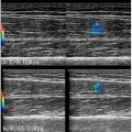
Here, we investigated the QUS analysis of two periodontal soft tissues (alveolar mucosa and gingiva) in vivo . The study cohort included 10 swine scanned at four oral quadrants, resulting in 40 scans. Two-parameter Burr and Nakagami models were employed for QUS-based speckle modeling. Parametric imaging of these parameters was also created using an optimal window size estimated in a separate phantom study.

Results

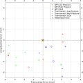
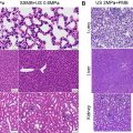
Phantom results suggested a window size of 10 wavelengths as the reasonable estimation kernel. The Burr power-law parameter and Nakagami shape factor were higher in gingiva than alveolar mucosa, while Burr and Nakagami scale factors were both lower in the gingiva. The difference between the two tissue types was statistically significant ( p < 0.0001). Linear classifications of these two tissue types using a 2-D parameter space of the Burr and Nakagami models resulted in a segmentation accuracy of 93.51% and 90.91%, respectively. Findings from histology-stained images showed that gingiva and alveolar mucosa had distinct underlying structures, with the gingiva showing a denser stain.

Conclusion

QUS results suggest that gingiva and alveolar mucosa can be differentiated using Burr and Nakagami parameters. We propose that QUS holds promising potential for the characterization of periodontal soft tissues and could become an objective and quantitative diagnostic tool for periodontology and implant dentistry to improve dental health care.

Introduction

Periodontal (gum) diseases are reported to affect nearly half (45.9%) of the adult population aged ≥30 years in the United States [ ]. These diseases involve various oral soft tissues that support and surround the teeth such as the marginal (free) gingiva, attached gingiva and alveolar mucosa, which are illustrated in Figure 1 for a swine model. The most prevalent periodontal diseases affecting these tissues are periodontitis and gingivitis, which are a continuum of inflammatory diseases. Periodontitis is initiated by bacterial infection, potentiated by inflammation, resulting in periodontal attachment loss of soft tissue from bone as well as actual bone loss. As periodontitis progresses, tooth loss is at risk of occurring. Periodontitis is also related to systemic diseases, such as cardiovascular diseases and diabetes. On the other hand, gingivitis is considered reversible as it involves gingival inflammation without clinical signs of bone loss [ ]. If oral diseases affecting both soft and hard tissues are not addressed at early stages they could cause immense pain as well as excessive economic burdens on the population—they were reported to have caused direct and indirect costs of as high as US$154.06 billion in the United States in 2018 [ ].

Bleeding on probing (BOP) is among the diagnostic modalities used in dentistry for the clinical assessment of soft tissue. BOP is an invasive method in which a probe marked with 1 mm ruler increments is inserted and gently pushed into the pocket/sulcus between the crown and the marginal (free) gingiva (see Fig. 1 ). Probe depth as well as potential bleeding are frequently recorded at office visits as a surrogate for gingival inflammation and are part of the standard of care, as BOP is a sign of periodontal inflammation. The normal probing depth is ≤3 mm, beyond which attachment/bone loss around a tooth is suspected. However, BOP has several limitations: it is invasive and often unpleasant for patients. Additionally, BOP is subjective, as the penetration force/insertion angle of the probe and tissue texture can vary readings significantly. Probe depth is also insensitive in the sense that it is only able to differentiate increments of 1 mm and small-scale penetration depths can be subjected to reading errors. Additionally, common variations in gingival thickness induced by different biotypes in different patients could increase the complexity of obtaining an objective assessment of inflammation by BOP [ ]. This method is qualitative as it describes either no, slight or profuse/spontaneous bleeding, and is a measure of tissue destruction at a late and already irreversible stage [ ]. It is noteworthy that although a lack of BOP observation is a strong indication of negative inflammation, BOP observations do not necessarily indicate the existence of underlying inflammation [ ].

Another traditional diagnostic method in dentistry is visual observation, which suffers from some of the same limitations as BOP. For example, swollen and erythematous tissue is indicative of periodontal inflammation. However, pigmented and thick tissue can mask these cardinal signs. Therefore, it is crucial to investigate non-invasive diagnostic modalities for an objective and quantitative characterization of oral soft tissues from a clinical workflow standpoint, as well as for improving public health and alleviating associated financial burden.

Toward this clinical goal, an imaging modality with promising potential for oral soft tissue characterization is ultrasound (US) imaging. As a non-invasive, non-ionizing, real-time, inexpensive and well-established modality, US has been employed in the imaging and characterization of various biological soft tissues such as the liver, thyroid, muscle, and so on, at differing depths and image resolutions [ ]. In dentistry, US brightness-mode (B-mode) imaging has been employed for lesion detection, gingiva thickness measurement and to delineate the surface of hard tissues (bone/crown) [ ]. Moreover, US-based elasticity estimations of oral soft tissues have been investigated in different studies [ , ]. US imaging offers information beyond B-mode imaging. One important aspect for US imaging is quantitative ultrasound (QUS). In the QUS analysis of tissues, the goal is to investigate quantitative parameters from uncompressed raw US scan data that can be linked to some measure of the underlying structure of tissues, which could offer clinical potential for tissue characterization [ , , ]. While B-mode images provide information on the landmark anatomical structures of tissues, they fail to provide information and contrast of the underlying soft tissue structure. QUS parameters could add more information to B-mode images, represented as a parametric image overlay. Although QUS analysis has been extensively applied to characterize various biological tissues , it has never been applied in clinical periodontics for soft tissue characterization and there are only a few studies with limited analysis involving QUS for periodontal soft tissue. For example, in the study reported by Di Stasio et al. [ ], US B-scan echogenicity in layers of oral soft tissues was compared using a measure of echo levels, but the employed method for the attenuation estimation deviated from standard techniques used to analyze US image echogenicity parameters quantitatively. Potential applications of QUS in periodontology include tissue characterization (i.e., gingiva vs. mucosa), tracking inflammation progress, automatic lesion detection, and tissue healing quantification. QUS could potentially complement BOP and other diagnostic tools for improved and more accurate characterization of periodontal tissues.

One class of QUS analysis in the medical imaging of tissues is focused on modeling the first-order statistics of US speckles. Speckles are granular (gray) textures observed in B-mode tissue images [ ] that result from the interference of back-scattered waves echoed back from various tissue scatterers close to each other during US pulse-echo imaging. Although speckles have a negative impact on B-mode image quality and are filtered out for US image representation, speckle patterns could incorporate information about underlying tissue structure and thus, could have clinical significance. Modeling US speckle statistics may result in the derivation of quantitative parameters that can be correlated with tissue pathology not visible on B-mode images. A number of well-established distributions for speckle modeling in QUS include Rayleigh , Homodyned-K [ ], Nakagami [ ] and, more recently, the Burr model [ ]. All of these distributions have been widely used in QUS-based tissue characterization. However, to the best of our knowledge, characterization of periodontal soft tissues using speckle modeling and these well-established distributions have not been reported in the literature.

Here, we aim to characterize periodontal soft tissue by investigating US speckle statistics using the Burr and Nakagami models in an in vivo animal study on swine oral tissues. Moreover, we present parametric imaging of these QUS parameters as additional information to that of B-mode images. Additionally, histological images of swine oral tissues were acquired using Masson’s trichrome and hematoxylin and eosin (H&E) stains with 20× magnification microscopy imaging to compare gingival and alveolar mucosal tissue structures with QUS analysis. QUS-based parametric imaging may have the potential to be used as an augmented tool for current imaging modalities in dentistry, such as cone beam computed tomography, to further aid oral surgeons and provide diagnostic value for clinical assessment in oral examinations.

Before we delve into QUS analysis, we will first present a concise overview of oral soft tissue anatomy to introduce necessary information and terms used within the rest of the paper.

Oral soft tissues: anatomy

Oral soft tissues are comprised of various components such as gingiva, alveolar mucosa, buccal mucosa and epithelium, each with different physiological properties suitable for a particular function during the mastication (chewing) process. The gingiva (G) and alveolar mucosa (M) are located closely in the proximity of teeth (crowns); however, the two tissues types are distinct and have a differing ultrastructure. Gingiva and alveolar mucosa are considered two important components of oral soft tissues that have drawn significant clinical studies due to the frequent occurrence of dental issues associated with qualitative and/or quantitative changes in gingiva and alveolar mucosa tissues [ ]. These tissues, along with other structures of hard and soft tissues, are illustrated in a swine model shown in Figure 1 .

Gingiva

The gingiva is a dense fibrous connective tissue with load-bearing intracellular layers, and its primary role is to protect the root and alveolar bone from deformation and degradation. The gingiva is covered by an additional highly keratinized layer called the epithelium (E) that forms a biological seal around the gingiva, lowering the penetration of some substances into the oral soft tissues beneath it .Connective tissues within the gingiva are mostly comprised of collagen fibers organized in different patterns: (i) thick collagen fibers arranged densely, and (ii) short and thin collagen fibers arranged sparsely along with fine-sized network (reticular) structures of fibers as well as some diffuse collagen fiber patterns [ ]. The gingiva comprises various fiber arrangements, as illustrated in Figure 1 , which include: alveologingival fibers (originating from the bone to the epithelium), dentogingival fibers (stretched from the tooth root to the gingival region), circumferential fibers (encompassing the tooth) and dentoperiosteal fibers (from the tooth root to the bone). In terms of vasculature, the gingiva has dense capillary vessels (≥15 pm in diameter) that are mostly perpendicular to the gingival surface and lack connective vessels, with sparse large vessels at a higher depth [ ]. The gingiva consists of two main parts: (i) the free gingiva, which wraps around the tooth and is free (not attached) from one side, and (ii) the attached gingiva, which is attached to the free gingiva from one side and is firmly connected to the alveolar bone on the other side. Among periodontal soft tissue, the gingiva has relatively higher exposure to external mechanical forces (cyclic and non-cyclic) applied during mastication compared with other oral soft tissues, and thus, has a stiffer nature [ ].

Alveolar mucosa

The alveolar mucosa is a membrane that lines the bone. Unlike the gingiva, the alveolar mucosa is less exposed to abrasive forces and is mainly non-keratinized. The alveolar mucosa has a higher level of elastic fibers, which makes it more elastic compared with the gingiva. The gingiva contains higher cross-linked collagen fiber levels and possesses some resistance to tensile loads. These elastic fibers tend to make the alveolar mucosa return to a resting state after being extended. Moreover, the alveolar mucosa is distinguished by a higher blood vessel supply ranging from capillaries to larger vessels and appears pinkish compared with the gingiva’s brighter white-pink color [ ]. The interstitial fluid within the vasculature provides cushioning when the tissue is under large masticatory loads.

Theory

In QUS, first-order speckle statistics is the probability distribution of the envelope of US echo amplitudes. Modeling speckle statistics could provide information on scatterer structure within tissues. This section provides the theoretical background for modeling first-order US speckle statistics as well as QUS parametric imaging using the Burr and Nakagami models.

The Burr model for speckle statistics modeling

A new framework has recently been proposed to model the first-order statistics of US echo amplitude from tissue backscattering that is based on a key assumption that scatterers within tissues are multi-scale fractal and their number density follows a power-law distribution with the characteristic size of scatterers (as the key power-law parameter related to scatterer density). The mathematics under this framework resulted in the Burr distribution model for describing the first-order statistics of US echo amplitude, which was the first application of the Burr model within the area of medical imaging [ ]. The Burr distribution was first derived in the 1940s without any implications for the field of US medical imaging [ ]. This framework was initially employed to describe US speckle statistics from in vivo livers in normal and abnormal conditions [ , ], as well as for describing speckle statistics from a set of simulated scattering structures in the form of cylindrical and spherical scatterers in which the number densities of multi-scale scatterers followed a power-law distribution with radii [ , , ]. The results from these studies showed that the Burr distribution successfully and efficiently described US speckle statistics. Later, the Burr distribution was employed in optical coherence tomography scans, where it was reported that the Burr distribution showed promising results in modeling speckle statistics [ , ]. Under this framework, the histogram of backscattered echo amplitudes (A) could be modeled as a probability density function (PDF), denoted as P(A) in eqn (1) with two underlying parameters: the key power-law parameter, b , and a scale factor, l , as follows:

P(A)=2A(b−1)l2[(Al)2+1)]b P(A)=2A(b−1)l2[(Al)2+1)]b

Burr b is associated with the number density of scatterers and increases with it, while Burr l is related to the echo amplitude and is elevated in tissues with higher echogenicity. These parameters provide additional information about the tissue’s underlying structure compared with the gray-scale B-scan alone. Burr b and l have shown potential in characterizing liver tissues in fibrotic versus normal conditions [ , ]. To estimate the Burr parameters from the tissue backscatter within a selected region of interest (ROI), we fit the echo envelope PDF of the speckle data to eqn (1) and derive the underlying parameters. Additionally, the Burr parameters can be estimated locally from the local speckle data statistics using a sliding window approach, where the ROI is swept by a small kernel and a local estimation map of the Burr parameters is calculated. To do so, we can utilize relationships between one or multiple statistical moments of the echo amplitude and the Burr parameters to determine a system of two equations with two unknown parameters [ ]. One statistic to employ is the first moment of the echo amplitude, i.e. , mean, denoted as E [ A ] and reported in eqn (2) . Other statistics could be the ratio of the square of the first moment of the echo amplitude, ( E [ A ]) ² , to the first moment of the echo intensity, E [ A ² ], as shown in eqn (3) . While eqn (2) shows that the first moment depends on both b and l , per eqn (3) the moments ratio depends only on a single parameter, ( b ). To estimate these two parameters, first b is obtained from eqn (3) and then it is plugged into eqn (2) to estimate l . The Burr scale factor, l , in eqn (2) is constrained by the finite value of b (measure of the scatterer number density from eqn [ ]) and by the value of the first moment of the amplitude (mean), E [ A ]. Using these two equations, one can obtain local estimations of the Burr parameters.

E[A]=(b−1)lπΓ(b−32)2Γ(b) E[A]=(b−1)lπΓ(b−32)2Γ(b)

(E[A])2E[A2]=(b−2)π(Γ(b−32))24(Γ(b−1))2 (E[A])2E[A2]=(b−2)π(Γ(b−32))24(Γ(b−1))2

Nakagami distribution

The probability distribution of the echo amplitude envelope from the two-parameter Nakagami distribution is modeled according to eqn (4) , where m is the Nakagami shape parameter and Ω is the Nakagami scale factor. These two parameters are estimated statistically from eqns (5) and ( 6 ). It is noted that the Nakagami m parameter determines the form of the speckle statistics PDF: if m <1, it is pre-Rayleigh and a heavy-tailed distribution; if m = 1, it corresponds to Rayleigh behavior; if m >1, it demonstrates a post-Rayleigh distribution [ ]. The Nakagami scale factor, Ω, represents the total intensity of the backscattered echo within the region under analysis.

f(r)=2mmr2m−1Γ(m)Ωme−mΩr2U(r) f(r)=2mmr2m−1Γ(m)Ωme−mΩr2U(r)

m=(E[A2])2E[A2−E[A2]]2 m=(E[A2])2E[A2−E[A2]]2

Ω=E[A2] Ω=E[A2]

Only gold members can continue reading. Log In or Register to continue