Abstract
Objective
Accurately measuring intracardiac flow patterns could provide insights into cardiac disease pathophysiology, potentially enhancing diagnostic and prognostic capabilities. This study aims to validate Echo-Particle Image Velocimetry (echoPIV) for in vivo left ventricular intracardiac flow imaging against 4D flow MRI.
Methods
We acquired high frame rate contrast-enhanced ultrasound images from three standard apical views of 26 patients who required cardiac MRI. 4D flow MRI was obtained for each patient. Only echo image planes with sufficient quality and alignment with MRI were included for validation. Regional velocity, kinetic energy ( KE ) and viscous energy loss ( EL ˙ ) were compared between modalities using normalized mean absolute error (NMAE), cosine similarity and Bland–Altman analysis.
Results
Among 24 included apical view acquisitions, we observed good correspondence between echoPIV and MRI regarding spatial flow patterns and vortex traces. The velocity profile at base-level (mitral valve) cross-section had cosine similarity of 0.92 ± 0.06 and NMAE of (14 ± 5)%. Peak spatial mean velocity differed by (3 ± 6) cm/s in systole and (6 ± 10) cm/s in diastole. The KE and rate of EL ˙ also revealed a high level of cosine similarity (0.89 ± 0.09 and 0.91 ± 0.06) with NMAE of (23 ± 7)% and (52 ± 16)%.
Conclusion
Given good B-mode image quality, echoPIV provides a reliable estimation of left ventricular flow, exhibiting spatial-temporal velocity distributions comparable to 4D flow MRI. Both modalities present respective strengths and limitations: echoPIV captured inter-beat variability and had higher temporal resolution, while MRI was more robust to patient BMI and anatomy.
Introduction
Quantification of intracardiac flow patterns may support diagnosis and understanding of various cardiac conditions, and assessment of underlying pathophysiology. Such information may help risk assessment, including predicting thrombus formation and gauging treatment effectiveness, as well as informing potential future treatment options. Recent studies suggested that cardiac hemodynamics are correlated to different types of cardiomyopathy [ ], including dilated cardiomyopathy [ , ]. At present, 4D flow MRI is the gold standard of intracardiac flow imaging, offering detailed 3D velocity vectors throughout the cardiac cycle for comprehensive quantification and visualization of cardiac blood flow patterns. However, it has practical limitations such as high costs, long scan durations and incompatibility with certain patient conditions or implants.
Echocardiography is a readily accessible, real-time imaging technique used extensively in clinical practice. Doppler ultrasound techniques enable the measurement of blood flow velocity through the valves [ , ], but only provide velocity information along the ultrasound beam direction, limiting assessment of complex, multi-directional flow patterns.
Echo-Particle Image Velocimetry (echoPIV) provides a 2D velocity field, revealing intracardiac hemodynamics [ , ]. EchoPIV based on conventional (low frame rate) imaging has explored the relationship between flow and heart diseases but is limited in quantifying the full velocity spectrum due to frame-rate limitations [ ]. High frame rate (HFR) echoPIV employs HFR contrast-enhanced ultrasound imaging to estimate blood flow patterns. HFR imaging uses diverging wave transmissions and software beamforming and allows imaging at 100× the frame rate of conventional echocardiography [ ]. In previous studies, echoPIV has been compared with optical PIV ( in vitro ) [ ] and pulse-wave Doppler ( in vivo ) [ , , ]. However, an in vivo validation for the whole intracardiac velocity field was still absent. Therefore, this study primarily aims to validate 2D echoPIV against 4D flow MRI for in vivo left ventricular flow imaging. Additionally, we examine the advantages and disadvantages of both imaging modalities. Finally, we report disturbed flow patterns in a patient with a severely dilated left ventricle (LV) and another one with left bundle branch block.
Methods
Setup of study and patient selection
Patients referred for cardiac MRI for screening of cardiomyopathy or determining the underlying etiology were selected. Exclusion criteria were hypertrophic cardiomyopathy, non-sinus rhythm and poor acoustic windows in conventional echocardiography. HFR echoPIV was acquired on the same day as cardiac MRI (except for one patient). This study was approved by the Erasmus MC Medical Ethic Review Committee (Rotterdam, the Netherlands), and written informed consent was obtained from all patients (METC-2018-057, NL63755.078.18).
4D flow MRI
Image acquisition was performed on a 1.5 T clinical MRI scanner (SIGNA Artist, GE Healthcare, Milwaukee, WI, USA) using an anterior phased-array coil. The protocol included breath-hold balanced steady-state free precession (bSSFP) cine images in the three standard long-axis views and a contiguous stack of short-axis images, all with 30 phases per cardiac cycle. Furthermore, a free-breathing, retrospectively ECG-gated 4D flow sequence with parameters shown in Table 1 was acquired directly after administration of gadolinium contrast agent (Gadovist 0.2 mmol/kg) prescribed in the axial plane covering the whole heart.
| Parameters | Value |
|---|---|
| Acceleration Method | HyperKat Factor 6 With Compressed Sensing |
| Flip angle (degrees) | 15 |
| Arrhythmia rejection | 30% |
| Respiratory compensation | 20% |
| Field of view (mm) | 380 |
| Phase field of view | 60%–100% |
| Repetition time (ms) | 4.2 |
| Number of excitations | 4 |
| Velocity encoding (cm/s) | 150 |
| Reconstructed number of phases | 30 |
| Acquired resolution (mm3) | 2 . 4 × 2 . 4 × 2 . 4 |
The 4D flow processing was performed using MASS software (Leiden University Medical Center, Leiden, the Netherlands) [ ]. A second-order plane fit was applied as a static-tissue interpolation offset correction to correct for phase-offset errors. The contours of the LV were delineated on 2D anatomical MRI sequences. To ensure precise alignment, the anatomical positions of these 2D slices were extracted from the DICOM data and were used to define matching cut-planes in the 4D Flow MRI volume. Flow data corresponding to these planes were subsequently exported from the 4D sequence and further processed using Matlab (R2019a, MathWorks, Natick, MA, USA).
Echocardiography
The echocardiographic protocol consisted of two parts: a standard clinical protocol using a clinical ultrasound machine (EPIQ 7 with probe X5-1, Philips Healthcare, Best, the Netherlands, f c = 2.5 MHz ); and the HFR contrast-enhanced ultrasound recordings using a research ultrasound machine (Vantage256, Verasonics, Kirkland, WA, USA) with a phased-array probe (P4-1, ATL, Bothell, WA, USA, f c = 1.5 MHz ). The setup overview is shown in Figure 1 . The clinical protocol includes B-mode and color Doppler acquisitions in the apical two, three and four-chamber (A2C, A3C and A4C) views and pulsed-wave Doppler measurements at the mitral valve tips and the LV outflow tract (LVOT).

Following the clinical imaging protocol, a diluted solution (1:3) of ultrasound contrast agent (SonoVue, Bracco Imaging SpA, Milan, Italy) in saline was intravenously infused (1 mL/min) using a continuous infusion pump (VueJect BR-INF 100, Bracco Imaging SpA). Upon verification of contrast agent arrival in the LV, the imaging system was switched to the research ultrasound machine for HFR imaging. HFR data were obtained and beamformed with the setup described by Voorneveld et al. [ ], a detailed description can be found in supplementary data. The pulse repetition frequency was chosen to reach the physical limitation of imaging depth (3553–6012 Hz). Each acquisition captured a total of 3000 frames of data (∼2 . 5 s), allowing for the recording of at least two cardiac cycles.
EchoPIV processing
EchoPIV was performed using custom Matlab code (R2022a, MathWorks, Natick, MA, USA) and, in brief, involved subdividing each image into smaller blocks and tracking the HFR contrast-enhanced ultrasound speckle pattern over time to obtain the velocity information in each block. A more technical description is provided in the supplementary data [ , ]. The final frame rate (after pulse inversion, angular compounding and ensemble averaging) of the velocity data was ∼122 . 5 frames/s. The vector field obtained by echoPIV was interpolated onto a uniform cartesian grid for flow analysis.
Registration
For an accurate comparison of MRI and ultrasound flow fields, spatial and temporal registration between the modalities is required. Temporal registration involved up-sampling the time series of MRI measurements (30 frames/cardiac cycle) to match the frame rate of the ultrasound images (∼100 frames/cardiac cycle). The R peaks of the ECG signals were used to separate echocardiographic acquisitions into cycles and to synchronize them with the retrospectively ECG-gated MRI data.
Spatial registration: MRI LV endocardial contours were manually drawn on the standard bSSFP long-axis cine images in each phase of the cardiac cycle using MASS. Given the assumption that the echocardiographic and MRI images represent the true, non-distorted dimensions and shapes of the LV, these contours were then spatially aligned (manually) to the ultrasound B-mode image by using a rigid transformation to ensure intrinsic anatomical and dimensional consistency. The same transformation was applied to the MRI vector field and the transformed 3D vectors were interpolated on the same grid as the ultrasound data and projected onto the 2D ultrasound plane.
Feasibility and assessment of registration
Inclusion criteria consisted of two aspects: (i) B-mode image quality, and (ii) co-registration of MRI and echocardiography. B-mode image quality indicates the clinical feasibility of echoPIV for flow estimation. Acquisitions with poor contrast/signal-to-noise ratio, blurred point spread function or bubble signal loss in the basal region were considered unfeasible and excluded from flow comparison.
Goodness of registration was quantitatively evaluated using the Dice coefficient between the end-diastolic LV endocardial MRI and ultrasound contours. We first excluded the acquisitions with severe foreshortening by setting a threshold on the Dice coefficient( > 0 . 85). Subsequently, we performed a visual assessment of all views by multiple independent observers (YH, JV, JGB) followed by a consensus session selection. This evaluation involved a careful visual comparison between the two modalities of key anatomical landmarks (the apical shape, septal wall, mitral valve and aortic valve, LVOT, and the position of papillary muscles) and the possible plane mismatch. The flowchart of the validation inclusion process is shown as part of Figure 1 .
Comparison of flow between EchoPIV and 4D flow MRI
We evaluated the spatial-temporal agreement of the two techniques using their velocity profiles, and commonly derived regional flow parameters: kinetic energy ( KE ), rate of energy loss ( EL ˙ ) and circulation, which are defined in the supplementary data.
The LV was split into basal, mid and apical regions by first selecting two basal points on the mitral anulus and a third point on the LV apex. The apex and the mid-point of the two basal points define the LV long axis. Two lines parallel to the line connecting the two basal points were then constructed that trisected the LV long axis, effectively dividing the LV into three segments: the base, mid and apex regions (see Fig. 1 ). In addition to these, we identified another parallel line at 1/9 of the LV long axis length for the mitral valve inflow. The velocity profiles were evaluated on the three parallel lines mentioned above—inflow, mid and apex. The flow comparison was performed over the whole LV as well as locally (in the basal, mid and apical regions of the LV). Two quantitative measures were used for comparison: Cosine Similarity (to assess similarity in the shape of the temporal pattern of each parameter between modalities) and normalized mean absolute error (NMAE, to assess absolute differences between parameters measured by each modality).
Statistical analysis
Statistical analysis was performed using Matlab Statistics and Machine Learning Toolbox. To evaluate the clinical characteristics of all study participants against those of the comparison group, a Student’s t -test was conducted for the continuous data and a Fisher’s exact test was conducted for the categorical data. p < 0 . 05 implied statistical significance. Student’s t -test was also applied to compare differences in Dice coefficient across three apical views. Bias and limits of agreement for temporal peak velocities between modalities, during systole and diastole, were estimated using Bland–Altman analysis [ ], reported with 95% confidence intervals (95% CI).
Results
Feasibility and assessment of registration
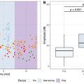
As shown in Figure 2 , among 78 standard apical view HFR acquisitions from 26 patients, 61 (78%) had sufficient B-mode image quality for echoPIV flow estimation and thus could be considered clinically feasible for echoPIV processing.

The mean Dice coefficient for all 78 acquisitions was 0 . 88 ± 0 . 05, indicating a high-level similarity between the end-diastolic echocardiographic and MRI masks. Dice coefficients for A4C, A3C and A2C (v.s. all views) showed no significant differences among the three types of standard apical views.
After removal of acquisitions that did not meet the stringent alignment criteria ( Movie S.6 – S.8 show examples of removed acquisitions), 24 acquisitions from 16 patients were selected for the quantitative flow comparison: 12 A4C, 6 A3C and 6 A2C views. A power analysis was conducted, indicating a minimum of 22 acquisitions were required to detect a peak velocity magnitude difference of 10% (CI was set to be 95%). This requirement was met by the size of the inclusion group.
Hemodynamic and echocardiographic data
General clinical, conventional echocardiographic and MRI characteristics for all patients and those included for comparison are displayed in Table 2 . No significant differences were found between the comparison group and the total patient group.
| Parameters | All Patients ( n = 26) | Comparison Group ( n = 16) | p Value |
|---|---|---|---|
| General characteristics | |||
| Age | 46 [19-76] | 39 [21-77] | 0.28 |
| Sex (male/female) | 17/9 | 9/7 | 0.74 |
| BMI | 24.8 (20.7-27.1) | 24.8 (20.2-26.7) | 0.69 |
| Heart rate (bpm) | 66 (57-74) | 72 (65-78) | 0.28 |
| Systolic blood pressure (mm Hg) | 123 (118-135) | 125 (118-136) | 0.63 |
| Diastolic blood pressure (mm Hg) | 73 (67-79) | 74 (67-77) | 0.84 |
| Echocardiographic characteristics | |||
| 2D LV end-diastolic volume (mL) | 187 (148-230) | 180 (133-198) | 0.93 |
| 2D LV end-systolic volume (mL) | 96 (72-128) | 81 (58-96) | 0.88 |
| LV end-diastolic diameter (mm) | 58 (54-62) | 56 (48-62) | 0.65 |
| Peak velocity E (m/s) | 0.7 (0.6-0.8) | 0.8 (0.6-0.9) | 0.19 |
| Peak velocity A (m/s) | 0.6 (0.5-0.7) | 0.6 (0.5-0.7) | 0.57 |
| E/A | 1.0 (0.8-1.4) | 1.3 (1.0-1.5) | 0.25 |
| E/e’ | 7.5 (6.4-10.0) | 7.1 (6.4-11.5) | 0.92 |
| Peak velocity LVOT (m/s) | 1.0 (0.6-1.3) | 1.0 (0.6-1.3) | 0.84 |
| LV ejection fraction (%) | 53 (40-56) | 55 (49-59) | 0.33 |
| MRI characteristics | |||
| LV end-diastolic volume (mL) | 204 (166-239) | 195 (164-226) | 0.92 |
| LV end-systolic volume (mL) | 120 (72-128) | 81 (68-122) | 0.92 |
| LV ejection fraction (%) | 52 (41-55) | 52 (46-58) | 0.47 |
| LV ejection < 45% (n) | 10 | 4 | 0.51 |
| LV Mass (gr) | 126 (104-155) | 121 (93-137) | 0.45 |
Related posts:
 Strain Patterns With Ultrasound for Assessment of Abdominal Aortic Aneurysm Vessel Wall Biomechanics
 A Bioengineered Cathepsin B-sensitive Gas Vesicle Nanosystem That Responds With Increased Gray-level Intensity of Ultrasound Biomicroscopic Images
 Classification of Neoadjuvant Therapy Response in Patients With Colorectal Liver Metastases Using Contrast-Enhanced Ultrasound—With Histological Pathology as the Gold Standard
 Attenuation Measuring Ultrasound Shearwave Elastography (AMUSE) as Noninvasive Imaging Biomarker for Liver Acute Cellular Rejection
 Ultrasound and Gold Nanoparticles Improve Tissue Repair for Muscle Injury Caused by Snake Venom
 Perioperative Detection of Cerebral Fat Emboli From Bone Using High-Frequency Doppler Ultrasound
Stay updated, free articles. Join our Telegram channel

Full access? Get Clinical Tree


