Computed tomography

Chapter 35 Computed tomography

Introduction

Radiography produces 2D images of 3D objects; it is important to remember that they are shadow projections (Ex Umbris Eruditio). This inevitably means that structures are superimposed, and the structure that is the object of imaging may be obscured from view. To address this problem focal plane tomography was developed shortly after the First World War, blurring out layers above and below the region of interest to provide an image of the required structure, but again it is 2D and prone to equipment and operating problems. The ideal is a technique that allows for 3D rendition of images.

The advent of X-ray computed tomography (CT) has had a great impact on medical imaging, primarily because CT solves this fundamental limitation of radiography by eliminating the superimposition of imaged structures.

CT uses a rotating X-ray source coupled to a bank of detectors to produce diagnostic images of the body. The basic premise of CT is that the attenuation pattern of the X-rays can be measured during rotation and spatially located; the sum of attenuation at each point can then be calculated and displayed. Since its inception at the beginning of the 1970s CT has now become a major technique in the routine diagnosis of disease, and scanners can be found in almost all district general hospitals (DGHs) in the UK.

Advantages of CT include

• Axial acquisition of cross-sectional images: with modern isotropic imaging, data can be post processed into multiple planes or rendered volumes, producing 2D or 3D images. Magnetic resonance (MR) is truly multiplanar, as scans are acquired directly in different planes without the need for reconstruction; however, the quality of CT isotropic reconstructions is high.

• Cross-sectional imaging has excellent low-contrast resolution (LCR), which is superior to other imaging methods with the exception of MR, which matches and in some cases exceeds the LCR of CT.

• CT images also show good high-contrast (spatial) resolution and excellent bone detail. MR does not image bone directly owing to the lack of free hydrogen within cortical bone.

• Digital imaging: this enables the manipulation of images, as well as post processing to other planes; the applied algorithm and windows can be adjusted to better visualise specific tissues. The application of filters and digital processing can enhance content, e.g. the use of edge enhancement for looking at bone.

• CT is generally well tolerated by patients, certainly more so than MR, which is less well tolerated owing to noise and claustrophobia. Contraindications for MR due to safety requirements do not apply to CT.

• CT is still more readily available than MRI and radionuclide imaging (RNI), being in situ in the vast majority of DGHs in the UK.

Disadvantages of CT include

• Ionising radiation dose: CT is undeniably an extremely high-dose technique, many examinations being among the highest, if not the highest doses, in use in medical imaging. Multiple examinations may approach the thresholds for deterministic radiation effects.

• Metallic artefacts cause loss of image detail; on many modern scanners this effect is much reduced by software corrections.

• Soft tissue structures surrounded closely by bone can be difficult to image, e.g. in the posterior fossa, where the soft tissue contrast of MR is superior. This is again a problem largely overcome in the latest generation of scanners.

• Misregistration artefact can be caused by relative movement of the body structures from the acquisition of a single slice to the next, e.g. due to inconsistencies in the patient’s respiratory pattern. If misregistration occurs then the reconstruction will be meaningless, as the same portion of anatomy could be portrayed at different positions in the reconstructed image. With the advent of single breath-hold scanning this is now less of a consideration. However, many centres, when scanning two areas such as the chest and upper abdomen, will overlap the two acquisition blocks to ensure no loss of information due to breathing differences between the two acquisitions. The dose implications of this technique are worthy of consideration.

In some quarters there is an attitude that CT can be undertaken by anybody, including non-radiographically qualified staff such as departmental assistants. It can be argued, however, that, along with every other branch of imaging, CT is operator dependent. Image quality is dependent on factors that should be adjusted for each examination, and more importantly, for each patient. In addition, because of the high dose burden all operators of CT equipment should be trained and skilled in optimising CT examinations;¹ indeed, specific additional training requirements are mandatory in some countries, such as the USA;² unfortunately, the need for requirements such as this can be only too evident.³

Equipment chronology

1874 Sir William Crookes constructs the cathode discharge tube. During his experiments over the next few years he discovers fogging of photographic plates stored near discharge tubes.

1895 Wilhelm Roentgen discovers X-rays while investigating gas discharge using a Crookes’ tube.

1935 Grossman coins the term ‘tomography’ to describe his apparatus for looking at detail in the lungs.⁴

1951 Godfrey Hounsfield starts work at EMI, initially working on early computers.

1956 Ronald Bracewell uses Fourier transforms to reconstruct solar images. At the same time Alan Cormack starts to work on solving ‘line integrals’.

1958 Korenblyum and colleagues in Ukraine work on obtaining thin-section X-ray images using mathematical reconstructions.

1961 William Oldendorf produces an image of the internal structure of a test object using a rotating object. He was unable to make further progress owing to the lack of available equipment to provide the computation that would have been required.

1963 Cormack publishes a paper on mathematical reconstruction methods.

1965 David Kuhl, one of the pioneers of RNI, produces a transmission image using a radioactive source coupled to a detector.⁵

1967 Bracewell produces a mathematical solution for reconstruction with fewer errors and artefact than found with Fourier.

Hounsfield and Ambrose come together to develop CT head scanning. Hounsfield uses an iterative algebraic technique rather than more complex mathematical formulae.

1971 The first clinical CT scanner is installed at Atkinson Morley Hospital under the supervision of James Ambrose. The first patient is scanned on 1 October. The first scanners were somewhat crude and took several minutes to produce each slice, which were of fairly poor quality. However, at the time even these crude images were revolutionary, enabling a first non-invasive glimpse at the soft tissue contents of the skull.

1972 Ambrose and Hounsfield discuss the clinical use of CT at the British Institute of Radiology annual conference.⁶ Clinical images are shown at RSNA.

1973 Hounsfield and Ambrose publish papers describing the design and clinical applications of the CT system.^7,⁸ EMI scanner becomes commercially available.

Hounsfield starts work on the second-generation scanner.

1974 Hounsfield produces abdominal images with a 20-second acquisition time.

1975 EMI CT 1010 second-generation scanner becomes available, soon to be followed by the CT 5005 – the first EMI body scanner.

In the next few years third-generation scanners become available but have problems with artefact, a problem solved by General Electric (GE). Fourth-generation scanners were later introduced to avoid the artefact problems initially suffered by the third-generation machines.

1979 Hounsfield and Cormack are awarded the Nobel prize for medicine.

1983 The first 2-second scanner introduced by GE (CT 9800).

1985 Electron beam CT developed.

1989 Siemens introduce spiral (helical) CT, using slip ring technology to enable the tube to rotate continuously without the need to go back to unwind its cables.

1992 Elscint Twin scans two slices simultaneously, which is a return to a method used by the original EMI scanners.

1998 Multislice CT initially incorporating four slices is introduced; GE, Picker, Siemens and Toshiba displayed systems at RSNA. Since then 8-, 16-, 32-, 40-, 64- and 128-slice machines have become available. Sub-second scan times enable body areas to be scanned in a single breath-hold. Advancements have in many cases had to await the development of computer systems robust enough to cope with the huge quantities of data generated, a problem initially encountered by Oldendorf.

2005 Siemens launch dual-energy scanners, opening the way to characterisation of chemical make-up of materials via simultaneous imaging at different kV values.

2007 Toshiba launch Aquilion One, 320-slice, ending the numbers game? Enables single rotation imaging of entire organs due to 16 cm coverage.

As mentioned above, CT systems have been classified according to the motion of the X-ray tube and detectors during scanning. There have been several generations of CT scanner, which are described here in brief.

First-generation scanner (Fig. 35.1)

The first-generation CT scanner used a single pencil beam of X-rays being measured by a single detector. In order to cover the area of interest, the movement required is a combination of translation and rotation. In the initial position, the tube/detector assembly moves across the scan field of view (translation) and a series of measurements of transmitted intensity are made. It then rotates 1° to its next position before commencing another translation.

Figure 35.1 Schematic of first-generation scanner.

This is a very time-consuming method and typical scan times were of the order of 4–6 minutes per slice acquisition. The early scanners attempted to compensate by having two detectors to perform two slices at once, a technique now resurrected in the latest generation of spiral scanners that offer ‘new’ multislice acquisition.

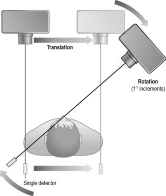
• Advantages: it was the first of its kind and offered the first opportunity for axial imaging of the head

• Disadvantages: mechanically complex, slow scans, which were only practical for scanning the head of patients who could be adequately immobilised using a water bag. The water bag was used to reduce the range of information required, as its density is closer to air than to that of tissue

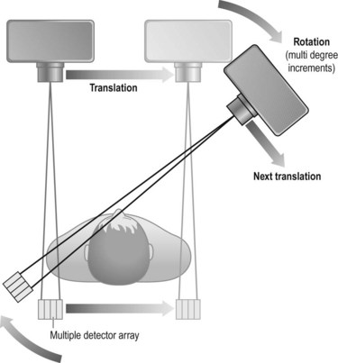
Second-generation scanner (Fig. 35.2)

The second generation used the same principles of movement as the first, i.e. a combination of translation and rotation, but used several new innovations. Instead of a pencil beam a narrow fan beam was now used, being measured by a bank of detectors. The fan beam is still not sufficient to cover the entire area of interest, so translation and then rotation is still required, but because more information is being gathered at each position, multiple degree rotational incrementation is possible.

• Advantages: as several detectors were being used, scanning times were significantly reduced and quality was increased. Typical scan times of the order of 20–80 seconds per slice were achievable. Again, two slices were acquired simultaneously on the EMI 1010 with a fixed slice thickness of 13 mm

• Disadvantages: the maintenance of the translate–rotate movement renders these scanners still mechanically complex

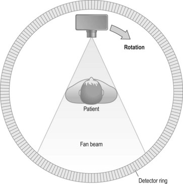
Figure 35.2 Schematic of second-generation scanner.

Third-generation scanner (Fig. 35.3)

Also known as a rotate–rotate scanner, this model was the first to do away with the requirement for translation across the patient by using a wide fan beam of X-rays. A large number of detectors (up to 1000) are used to allow for the increased beam width, and the tube and detectors are rigidly coupled and rotate jointly about the patient. Rotation only is required, as the fan beam covers the entire body. It is this configuration that is still the most commonly used, even in the latest multislice equipment.

• Advantages: the greater number of detectors plus the rotation-only movement allows shorter scan times, typically of the order of 2–8 seconds. The width of the fan beam can be adjusted (collimated) to limit the beam to the area under examination. Use of the rotation-only movement renders this type of unit mechanically simpler than its predecessors

• Disadvantages: detectors were expensive, therefore more detectors equals more cost. Also more processing power is required, as more information is gathered at one time. Initially problems were encountered with circular artefacts, but this was overcome by adjusting the detectors

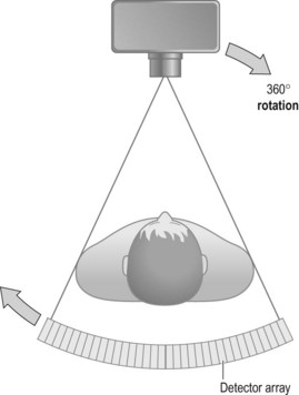
Figure 35.3 Schematic of third-generation scanner.

Fourth-generation scanner (Fig. 35.4)

This scanner was similar to the third-generation scanner, again using a wide fan beam but with a complete circle of detectors around the patient. In this case only the tube rotates, the detector ring being stationary.

• Advantages: mechanically simpler owing to having fewer moving parts. Scan times reduced and now taking 1–10 seconds

• Disadvantages: the high number of detectors equals high cost. There were also greater calibration difficulties. As the tube is rotating within the detector ring, the detectors are further away from the patient, leading to a greater penumbral effect

Figure 35.4 Schematic of fourth-generation scanner.

Electron beam computed tomography (EBCT)

A completely different concept, the electron beam is directed to the anode rotating around the patient, and is again linked to a bank of detectors. As mechanical rotational movement is now not used, quick (50 ms) scans are possible. EBCT has been used for gated cardiac studies for some time. For several years this was the only CT technology that could provide high-quality cardiac imaging, but now commonly available multislice and dual-source equipment can match EBCT in cardiac studies.

Spiral/helical CT

Helical scanners are also described as volume acquisition or spiral scanners, so for clarity the term helical will be used throughout this chapter.

In the 1990s ‘conventional’ CT began to be replaced by helical scanners. Owing to cost, availability and equipment replacement programmes, it was only in the late 1990s that these became the norm in the UK. Ironically, this occurred just as this technology itself was superseded by the introduction of multislice helical scanning.

Helical scanning differs from conventional CT in the method of data acquisition. Instead of a single 360° rotation that produces a single slice followed by an incremental table movement, in helical scanning a volume of data is acquired.

One of the main advantages of this method of continuous data acquisition is its speed. As a large volume of data can be acquired very rapidly, a series of images that would take several minutes to acquire in conventional ‘slice by slice’ mode can now be obtained in seconds.

This is due to both the use of slip ring technology, enabling continuous rotation of the X-ray tube around the gantry (without the cables, which previously had to be ‘unwound’ by a return rotation prior to the next slice being obtained), and improvements in the design of the tube and its drive motors enabling sub-second acquisition times.

This rapid data acquisition means that large areas of the patient can be imaged within a single breath-hold, eliminating one of the major problems for image reconstruction and interpretation: misregistration. Respiratory misregistration can be completely eliminated, and the short scan times make it less likely that patient movement becomes a factor.

Multislice CT

The latest advance in scanner design is the multidetector volume acquisition scanner, ironically a return to one of the features of the original EMI scanner – multiple detector arrays. The difference is that the first EMI scanner had two rows of one detector, whereas the latest multislice scanners have tens of thousands of detector elements. The majority of scanners are of the third-generation type with rotating tube and detector array.

Large volumes can be rapidly imaged with thin slice widths, enhancing the diagnostic capacity of CT. Large numbers of thin slices can be reconstructed to produce high-quality volume rendered images, with the elimination of ‘stair step’ artefacts and the reduction of partial volume artefacts.

Advantages of multislice include

• Speed of acquisition – sub-second rotation speeds are now the norm

• Compared to single-slice helical, multislice enables the same acquisition in a shorter time, or larger volumes to be scanned in the same time, or thinner slices to be scanned

• All manufacturers have sub-millimetre scan capabilities. Toshiba have detectors that are 0.5 mm, matching the pixel size to produce a voxel which is the same size in each dimension: termed isotropic (see Fig. 35.10). Isotropic and near isotropic voxels enhance the 2D reformatting ability of the scanner, enabling high-quality multiplanar reconstructions from an axial data set. 3D reformats produced are also excellent, with none of the problems of possible misregistration and information loss inherent in MR owing to its longer scan times.

Equipment

The X-ray tube

The advent of spiral scanning with its continuous rotation means that huge demands are placed on the X-ray tube used in modern scanners. The tube needs to provide high output while effectively dissipating the heat produced. Air conditioning is generally required to maintain a comfortable temperature in the scan room and to assist with heat dissipation. Large anode discs in metal or ceramic tube envelopes are common, the anode usually being mostly graphite with a tungsten/rhenium target track.

Beam shaping filter

In any CT scanner the X-ray beam produced is in fact heterogeneous, having a range of energies. Filters are applied to the beam on exiting the tube to reduce the range of energies. Filters also shape the beam to produce a more uniform result at the detectors in order to reduce the dynamic range required in the detector electronics.

Collimators

In a single-slice system a pre-patient collimator will limit the beam to the prescribed slice width at the centre of rotation; a post-patient collimator will then limit the beam incident on the detectors to the slice width. For example, pre-patient collimation to 4 mm will result in a 4 mm slice being produced.

In a multislice system the beam is again collimated at the centre of rotation but the result will differ. For example, in a four-slice system the 4 mm collimation given above will result in 4 × 1 mm slices being obtained.

Table

The table is an important element in CT. They are usually of carbon fibre construction with rise and fall action; this gives strength without interfering with the resultant image, and facilitates patient handling. The table must be able to provide a wide range of movement at various speeds. Accuracy of movement is vital, as any inconsistency would have detrimental effects on the image produced.

Table-tops are generally curved, except for those tables used in radiotherapy planning, where a flat table-top is essential to allow CT simulation. Simulation needs to reproduce accurately the patient’s position on the flat treatment table. Consequently, scanners used for both purposes will often have interchangeable table-tops for diagnostic and planning sessions.

Detectors

Modern detectors are of the solid state type, mostly using ultrafast ceramic detector elements. An incident beam causes scintillation; the photon produced is then converted to an electrical signal by a photodiode and sent on to the electronics. The detector array is formed by a series of individual elements, as shown in Figure 35.5.

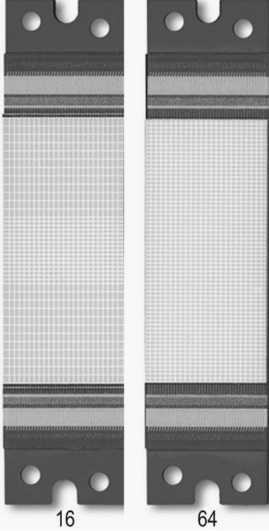
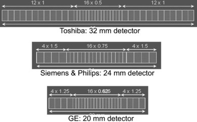
Figure 35.5 Aquilion 16 and 64 detector arrays. Both provide up to 32 mm coverage per rotation. The 16-slice detector has 16 × 0.5 mm elements centrally, with 12 × 1 mm elements either side, enabling acquisition of 16 × 0.5 mm or 16 × 1 mm or 16 × 2 mm slices per rotation. The 64-slice detector provides 64 × 0.5 mm slices per rotation.

Reproduced with permission from Toshiba.

Different manufacturers have differing approaches to the format of detector arrays, with four-slice machines being available as fixed matrix, adaptive or mixed arrays. Each of the major manufacturers has taken a different approach to 16-slice, and as can be seen in Figure 35.6, the choice of array format affects the minimum slice width available, the number of slices available at minimum width, and the range of slice widths available.

Figure 35.6 Comparison of 16-slice detector arrays.

Data acquisition system (DAS)

The DAS ‘reads’ the measurements from the detector array, converts these analogue signals into digital format, and transmits the digital signal to the computer systems for reconstruction into the presented images.

The DAS needs to be able to deal rapidly with a vast amount of data being generated every second; in current computing technology there is a limit to how much data can be handled at the necessary transfer rates. Development of these systems is advancing rapidly, but they have been a limiting factor to the speed of development of larger multislice arrays.

Computer system

The computer system processes operator input to set scanning parameters, patient information and archiving instructions. It also receives the information from the DAS which is then processed to form the image. A wide range of post-processing options are available on modern scanners which again take place within this system, or alternatively on dedicated workstations. High-speed high-capacity computers are required to perform these tasks at speeds that were unthought of until relatively recently.

Archiving requires some consideration; although archiving systems have increased greatly in capacity (and decreased in cost) in recent years the amount of data generated has followed the same pattern. Only selected reconstructions are generally sent for storage and access on picture archiving and communication systems (PACS); raw data, if stored, is often on high-capacity optical discs.

Physical principles of scanning

What happens to a homogeneous X-ray beam as it passes through an object? The X-ray photons interact with the material through which they pass and are attenuated by it. If the intensity of the emerging beam is measured, we know the initial intensity and so the attenuation within the object can be measured.

With the X-ray tube of a CT scanner in one position, a narrow X-ray beam passes through the patient and the attenuation along the line taken by a particular beam through the patient can be calculated from the intensity of the emergent beam measured by a detector. The X-ray intensity transmitted through an object along a particular path contains information about all the material it has passed through, but does not allow the distribution of the material along the path to be discerned.

For the energies used in CT the attenuation of the beam is due to:

• Absorption: photoelectric

• Scattering: Compton (mainly)

Attenuation due to photoelectric absorption is strongly dependent on the atomic number of the material (αZ³).

Attenuation due to Compton scattering does not depend upon atomic number, but on the number of free electrons present. The number of electrons per gram of an absorber is remarkably constant over a wide range of materials; however, because their density varies considerably, the number of electrons per metre does show variation across a range of biological materials. It is this difference between attenuation processes that enables differentiation of chemical composition in dual-energy equipment.

If we consider the simplistic case of a homogeneous beam passing through the medium, the attenuation in the tissues follows the Lambert–Beer law, which states:

where µ = linear attenuation coefficient

I_o = original intensity

I = transmitted intensity

x = thickness of material.

In CT we are interested in measuring the linear attenuation coefficient (LAC). Solving the Lambert–Beer equation for LAC, we get:

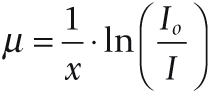
I is measured by the detectors, I_o and x are known, hence µ can be calculated.

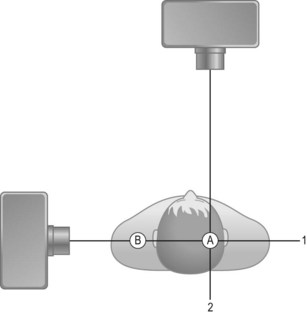
As mentioned earlier, the X-ray beam produced is in fact heterogeneous, having a range of energies. Filters are applied to the beam on exiting the tube to reduce the range of energies incident on the detector array.

Traditionally a narrow beam was required for accurate localisation of the attenuating tissues. Readings are taken from multiple angles to give a series of values of linear attenuation of the beam along intersecting lines through the patient. For example, in Figure 35.7 a bony object would have the same attenuating effect on ‘beam 1’ whether at position ‘A’ or ‘B’. However, from ‘beam 2’ it is possible to localise the structure to position ‘B’.

Figure 35.7 Localisation of position.

In general, then, the transmitted intensity depends on the sum of the attenuation coefficients for all points along the path of the beam. Thus the log transmission measurement is sometimes referred to as a ‘ray sum’ or ‘line integral’ of the attenuation along the path.

A radiograph can be considered to be composed of many such ray sums, produced unidirectionally, hence superimposing all structures encountered by the beam. Because of the differences in transmitted intensity, interfaces between bone, tissue and air are well demonstrated. The differences between adjacent soft tissues are not sufficient for good differentiation and so they are less well demonstrated.

To demonstrate soft tissues we need to eliminate superimposition by taking ray sums from multiple directions; these ray sum measurements can then be mathematically reconstructed to generate an axial image formed by estimating the distribution of the linear attenuation coefficient within the irradiated volume. The image produced can then be digitally manipulated to maximise contrast, enabling adequate visualisation of subtle changes in tissue density. The ability to produce such images is the main strength of CT as an imaging modality.

The information acquired by the detectors is passed to the computer. Once this data is committed to the computer memory it can be manipulated by the resident software to produce an image which is reconstructed on the screen of the viewing console. Reconstruction takes place via the application of a complex mathematical algorithm to the data obtained, usually a filtered back projection. Consideration of the detail of this mathematical process is beyond the scope of this chapter, but is well described in texts such as Seeram.⁹

Image reconstruction in its simplest form consists of recalling the digital information fed to the computer from the detectors via the DAS, and converting this information to an analogue voltage signal that controls the electron sweep within the display monitor.

Helical image reconstruction is more complex: because the table is continuously moving only one ray sum lies in the scan plane; the rest of the ‘slice’ information is interpolated from the acquired volume. 360° and 180° interpolations are used. As seen in Figure 35.8, a 360° interpolation requires data from two tube rotations for slice reconstruction. 180° interpolation allows smaller slice widths to be accurately reconstructed.

Figure 35.8 Diagrammatic representation of interpolation of helical data. 180° interpolation – X to X; 360° interpolation – 0 to 0.

Only gold members can continue reading. Log In or Register to continue

Stay updated, free articles. Join our Telegram channel

Tags: Medical Imaging Techniques, Reflection and Evaluation

Mar 3, 2016 | Posted by admin in GENERAL RADIOLOGY | Comments Off

Full access? Get Clinical Tree

Get Clinical Tree app for offline access

Get Clinical Tree app for offline access