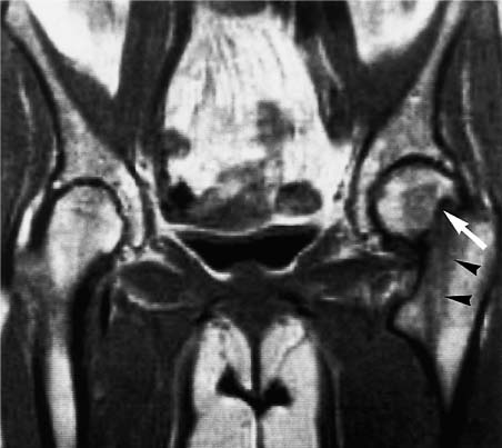
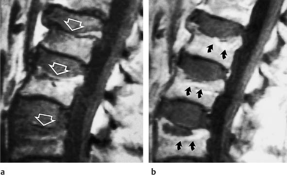
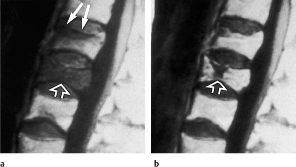
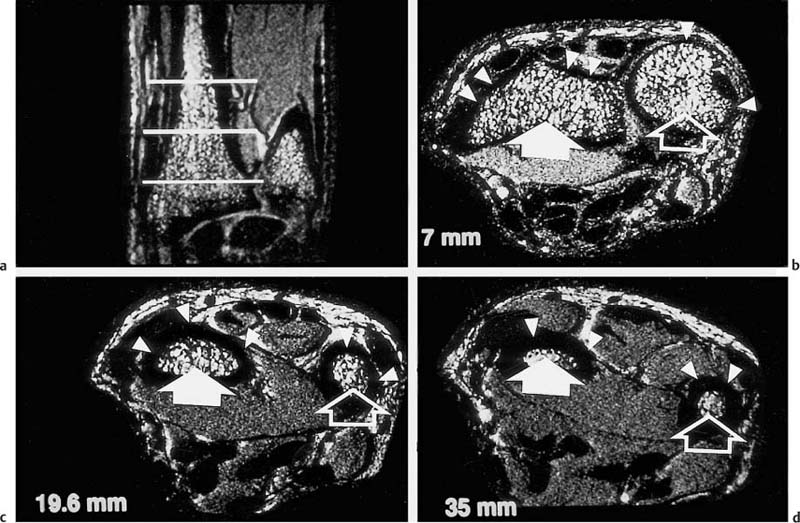
Osteoporosis

S. Grampp, M. Vahlensieck, P. Lang, and H. K. Genant

Introduction

Numerous techniques are currently available for diagnosing osteoporosis and osteoporotic fractures and for measuring osseous density and fracture risk (19). Most methods use ionizing radiation and calculate the bone mineral density (BMD) from the measured radiation absorption. In recent years, MRI has been used for diagnosing osteoporosis, with emphasis on visualizing osteoporotic deformities and fractures. High resolution techniques have been used to depict the internal osseous structures in order to make statements about their abnormalities in osteoporosis. Furthermore, the relaxation times (relaxometry) have been quantified to diagnose osteoporosis and to monitor its course (36 a, 42 a, 46 a, 49 a). Such quantification generally measures the effective T₂ time (T₂ *), sometimes expressed as its reciprocal value (1/T₂ *). So far, MRI cannot deliver the required low reproducibility of less than 2%, as achieved by other quantitative osteoporotic methods. This chapter presents the MRI evaluation of osteoporosis by discussing imaging and relaxometry separately.

MR Imaging of Osteoporosis

Osteoporotic Fractures

MRI can diagnose fractures that are undetectable on radiographs. Such radiologically occult fractures are relatively common in old osteoporotic patients. The detection of occult fractures of the proximal femur with MRI has been documented in several studies (12, 33, 38, 40, 52). MRI characteristically delineates the fracture line as markedly decreased signal intensity, surrounded by bone marrow edema. These changes are attributed to focal hyperemia and edema, impacted osseous trabeculae and reparative processes. MRI can diagnose osteoporotic insufficiency fractures of the pelvis, sacrum, hips and long tubular bones with a sensitivity that is at least comparable to and, according to some studies, even greater than scintigraphy (4, 5, 34). This is especially true during the few days following trauma (Fig. 13.1), when the findings of the bone scan often are still inconclusive.

MRI also makes a great clinical contribution by its ability to distinguish osteoporotic compression fractures of vertebral bodies from pathologic compression fracture due to underlying malignancy (1, 2, 42, 50, 53). Pathologic tumor-related fractures induce an abnormal signal pattern in the affected vertebral bodies (18, 35, 37), often accompanied by a convex deformity of the anterior and posterior margins of the vertebral bodies. The adjacent vertebral bodies frequently harbor metastases and show corresponding foci that have a low signal intensity on T₁-weighted and a high signal intensity on the T₂-weighted images. Osteoporotic fractures, in contrast, frequently show band-like signal changes, adjacent and parallel to the end plates. The nondeformed portions of the vertebral body exhibit a normal signal pattern (Fig. 13.2). Neighboring nonfractured vertebral bodies generally display a normal signal intensity in the bone marrow. For the differentiation between osteoporotic and pathologic vertebral compression fractures, MRI has a higher sensitivity than bone scintigraphy and a higher specificity than CT (1, 2, 50).

Fig. 13.1 MRI of the hip 8 hours after fracture of the femoral neck in a 76-year-old patient. The coronal GRE image shows a subcapital fracture line of low signal intensity (white arrow) with adjacent areas of moderate to low signal intensity (black arrowheads), corresponding to edema or hemorrhage.

Some studies have suggested that a distinction between osteoporotic and malignant vertebral collapse can be achieved with intravenous administration of contrast medium (9, 22). Osteoporotic vertebral collapse shows enhancement that is linear and parallel to the fracture line (Fig. 13.3), while malignant collapse generally shows patchy enhancement.

Fig. 13.2a, b Osteoporotic vertebral compression fractures.a Sagittal T₁-weighted image several days after the fracture. The L1 vertebral body shows a biconcave deformity (open arrow) and a low-signal marrow. In addition, the superior end plate of the T12 vertebral body is indented and shows a low signal intensity (arrows).b Sagittal T₁-weighted SE image several months after the fracture. Normalization of the signal pattern in the T12 vertebral body. The small area of decreased signal intensity in the L1 vertebral body (open arrow) corresponds to focal sclerosis.

Fig. 13.3a, b Osteoporotic compression fracture before and after administration of contrast medium.a The precontrast sagittal T₁-weighted SE image shows several compression fractures (open arrows) involving the L2–L4 lumbar vertebral bodies.b After administration of contrast medium, there is linear enhancement (curved arrows) parallel to the fracture lines in the affected vertebral bodies. This pattern is characteristic of osteoporotic fractures.

MRI has a limited ability to distinguish between acute traumatic and osteoporotic insufficiency fractures since either fracture produces localized signal changes caused by bleeding and reparative processes. Marked osseous deformity together with dislocated fragments is more often seen after acute trauma, while finding other collapsed vertebral bodies with a normal marrow signal pattern favors an osteoporotic origin.

The altered signal pattern of the bone marrow induced by a non-neoplastic fracture generally returns to normal within several months and only a deformed vertebral body remains.

High Resolution Imaging of the Trabecular Pattern

Besides measuring trabecular density and width, MRI can produce high resolution images that visualize the trabecular microstructure. After appropriate modification of the computer programs, standard MRI systems can generate images with a resolution of 78 × 78 × 300 µm for the finger phalanges (24) and of 78 × 78 × 700 µm for the distal radius (Fig. 13.4) and calcaneus (32).

Postprocessing using CT-derived techniques of image analysis (1, 8, 13, 24, 25, 36, 51) can yield quantitative parameters, such as the proportion of bone in a two-dimensional section, the average trabecular thickness, the number of trabecular branches and their preferred spatial orientation. When interpreting these parameters, one must be aware of erroneous calculations due to misregistrations introduced by incorrect separation of bone and marrow components, relatively limited spatial resolution or partial volume effects. Aside from these methods, additional techniques for image and structure analysis are available but will not be discussed in detail since they are largely still investigational. They include morphological granulometry (6), calculation of fractal elements (32), and wavelet processing (46). It is hoped that the quantitative analysis of the osseous morphology may predict the fracture risk better than the quantitative measurement of the bone density.

Fig. 13.4a–d Visualization of the distal radius with a 1.5 TSigna MRI system (General Electric, Milwaukee, USA). High resolution imaging with a T₂-weighted water presaturated GRASS sequence with sagittal thickness of 700 µm and a spatial resolution of 156 µm.a Coronal section through the distal forearm and wrist. The levels of the axial sections are marked as white lines on the coronal image.b Axial section about 7 mm distal to the cortical end plate of the radius (average T₂ * relaxation time in twelve healthy subjects = 18.02 msec [20]).c Axial section about 20 mm distal to the cortical end plate of the radius (T₂ * time = 21.20 msec).d Axial section about 35 mm distal to the cortical end plate of the radius (T₂