) is a vector that lines up with the external field  (the transverse components cancel each other out). Once the bulk magnetization has lined up with the external field, an RF field
  is applied to excite the nuclei. The frequency of the RF field is the same as the rate of precession of the nuclei (Larmor rate) so that energy from the excitation may be absorbed. Only the atoms that are precessing at the Larmor rate will be excited and reach a higher energy state. Once the RF field is removed, the nuclei begin to return to their original state, releasing energy in the process. The energy released in the transverse plane is known as the T1-signal and the energy released in the longitudinal plane is known as the T2-signal. Different tissues and pathologies have different T1-T2 relaxation times (which translates into different contrast in the output image). Because regions of the brain are composed of more or less water/fat, soft-tissue structures of the brain are imaged with good results.
The 3D position from which photons were released is learned by applying additional gradient fields during the scan. These strong magnetic field gradients cause the nuclei at different locations to rotate at different speeds and makes the magnetic field strength vary depending on the position within the patient. This in turn makes the frequency of released photons dependant on their original position in a predictable manner, and the original locations can be mathematically recovered from the resulting signal by the inverse Fourier transform. In other words, gradient fields selectively excite regions in the patient that are used to decode the corresponding pixels in the image.
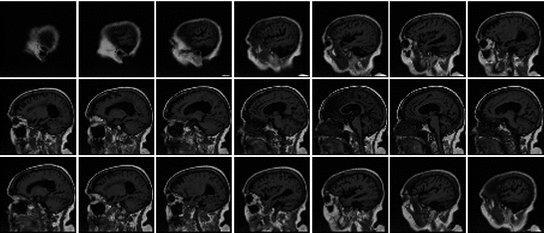
The result is a volumetric data set which offers a 3D representation of anatomy and pathology. Each image (slice) is acquired in a specific direction, which is parallel to an imaging plane. There are three perpendicular imaging planes that are most commonly used: axial (horizontal), sagittal and coronal. An example sagittal T1-weighted MR dataset, acquired from a single-coil scanner, is shown in Fig.
1.
The area the gradient field excites determines the resolution of the pixels (voxels) in the image, i.e., if a smaller area is excited, the resolution of the pixel in the final image increases. Slice thickness works the same way, i.e., if a large region in the z-direction (thick slice) is excited, the resolution in this dimension is low. It is possible to generate images of very high resolution, by exciting smaller and smaller volumes, except that this would require many more excitations and gradients to be applied, which significantly increases scan time.
Long acquisition times are a natural side effect of MR imaging. Each slice needs to be spatially encoded, which requires a series of excitations and during each excitation, a line in the Fourier domain (k-space) is acquired. Between excitations it is necessary to wait for the excited spins to return to equilibrium again (relaxation). Therefore, relaxation time and the number excitations have direct impact on the acquisition time.
In single-coil technologies, to speed up scanning, moderate values for the pixel height, width and slice thickness are usually chosen. Moreover, there is usually a gap left between adjacent slices, to facilitate even more efficient scanning times. Using larger volume elements creates faster scanning times at the expense of resolution. Resultantly, there have been many research efforts dedicated to overcoming the balance between resolution and scan time. For example, single-shot techniques such as Fast Low Angle SHot (FLASH) [
8] or Echo Planar Imaging (EPI) [
9]. The acquisition times of these techniques are significantly shorter, but the images are in general of lesser quality. They suffer from low signal-to-noise ratios (SNRs) and are very sensitive to the inhomogeneities of the main magnetic field [
10]. Details on single-coil technologies and the way they affect noise are discussed in the following section.
The latest and most innovative methods for speeding up acquisition times are achieved by sparsely sampling the k-space data (which reduces the number of required excitations). However, reduction of the sampling rate in the frequency domain (k-space) violates the Nyquist theorem of perfect reconstruction, and consequently there is aliasing in the spatial domain images. To compensate for the data loss in the spatial domain, multiple receiver coils and Parallel MRI (pMRI) reconstruction techniques can be used to recover the missing data.
The principle of pMRI is focused around the use of multiple receiver coils (phased-array coils or multicoil) to capture the image data [
11]. Each coil has a spatially varying sensitivity map that dictates the image reception profile of the coil. Moreover, each coil is positioned so that each has a different sensitivity over the the Field of View (FOV) [
12]. The distinct sensitivity profile of each coil is modulated with the pixel value of the image and since there are multiple sources capturing the same information, the missing k-space information can be calculated [
12]. Since these coils are working simultaneously, the introduction of redundancy gives way to a significant reduction in acquisition times. Details on pMRI and the way it affects noise in MRI are discussed in the next section.
1.2 Fluid Attenuation Inversion Recovery (FLAIR) MRI
To automatically analyze WML, Fluid Attenuation Inversion Recovery (FLAIR)-weighted MRI are used because of their ability to localize ischemic brain pathology. FLAIR images have very similar properties to T2-weighted images, in terms of tissue contrast characteristics. In T2-weighted images, water-filled tissues are imaged as bright or high-signal regions, whereas fatty tissues are represented with low intensities. This translates to dark gray and light gray intensities for white matter (WM) and gray matter (GM), high-intensity values for cerebrospinal fluid (CSF).
Most pathology is associated with increased water content [
4], so T2-weighted images highlight ischemic pathology such as WML. However, CSF also shows up as high-intensity signal in T2 images which reduces the discrimination of peri-ventricular WML (lesions close to the ventricles). FLAIR MRI overcomes these challenges by removing the T2 mobility so that the CSF signal is nulled (i.e., the intensity of CSF is set to zero).
1 This produces better discrimination of pathology [
4] since the CSF signal does not interfere with the signal of the hyperintense pathology (WML). Figure
2 contains the corresponding T2- and FLAIR weighted images for a patient with WML. The ventricular high signal material shown in the T2 images impede delineation of WML, whereas the CSF is dark in FLAIR MRI, providing much better visualization of white matter pathology.
The FLAIR modality has been used in many studies to detect the presence of white matter lesions and other neurodegenerative disorders [
4,
13,
14] due to its ability to localize pathology (as shown in Fig.
2). Therefore, this modality is an excellent candidate for the automatic detection and characterization of WML.
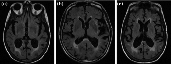
Some additional sample FLAIR MRI with varying lesion loads (total WML volume) are shown in Fig.
3. In each image, there are three major tissue classes in the cerebral region (excluding outer head structures):
CSF: darkest class in the image,
Brain (both GM and WM): comprised of medium intensity values,
WML: most intense objects (after brain extraction).
Normally, in MRI, WM and GM are clearly differentiable and compose two separate tissue classes. However, imaging parameters in FLAIR MRI cause GM and WM classes to have similar intensity values and thus are treated as a single class [
15]. Therefore, a tissue segmentation scheme for FLAIR MRI would search for estimates of the CSF, brain and WML classes, individually.
2 Challenges of Segmenting FLAIR MRI
Images with inherent artifacts may cause slight difficulty for human interpretation, but they can cause significant challenges for algorithms. A computer can easily tell the difference between two pixels’ intensity values, even if they only differ from one another by a few graylevel values. As a result, imaging artifacts can cause erroneous results in intensity-based segmentation schemes [
15], misclassified pixels in automated tissue classification algorithms [
16], inaccurate 3D reconstructions, etc. There are many noise sources in MRI that are produced by the imaging acquisition system.
Much research has gone into mathematically modeling the images’ noise fields in MRI and there are three main issues: acquisition noise [
17], the tissue nonuniformity issue [
18] and the PVA effect [
17]. Consider an undistorted, “clean” image

distorted by a multiplicative and additive noise source:
where

is the distorted image. In MR images

is known as the bias field or tissue nonuniformity artifact, and

is the additive (acquisition) noise field. The bias field is a smoothly varying field caused by inhomogeneity of the magnetic field [
19]. The bias field is not discussed in this work
2 so we set

. The additive noise source,

, is generated by acquisition noise from the system [
20] and must be considered in any automated MRI segmentation technique.
A third type of artifact is known as partial volume averaging (PVA) and it cannot be modeled with Eq.
1 as it has its own degradation model. In concerns the imaging of finite volume elements that have more than one tissue type/structure within the imaging section, pixel or voxel. The consequence is that the signals of the structure are averaged. As will be shown, PVA and acquisition noise are inherently related with one another, as well as the imaging system that is used to acquire the images. Handling these two artifacts is challenging but is required for accurate WML segmentations. These artifacts are discussed in this section to provide motivation for the proposed segmentation methodology.
2.1 Acquisition Noise
In MR images, the signal-to-noise ratio (SNR) is intrinsically related to the resolution of the images [
21]. As a result, the SNR of the output images may be modest or even low, making acquisition noise more apparent in the output image. Additive noise poses significant challenges for automated WML segmentation since it changes the intensity profile each tissue class; image classes are no longer clearly discernible in the intensity histogram and contrast between tissue classes is significantly reduced.
To combat the downfalls associated with acquisition noise, many researchers have investigated MRI noise characteristics and have tuned their processing technologies to these properties. This requires good knowledge of the acquisition process since noise in the output image is inherently related to the way the image is acquired. There are two dominant technologies used for MRI acquisition that depend on either single-coil technologies, or multicoil phased array systems. These two families create substantially different noise properties in the final image.
2.1.1 Single-Coil Technologies
Single-coil technologies use a single coil to transmit and receive NMR signals, which has direct bearing on the way noise is rendered in the image. It is well known that during acquisition the distribution of the noise within the single coil is Gaussian with zero mean and

standard deviation [
20–
23]. Each MR image (slice) is collected from the coil in the Fourier domain (k-space), which is inverted through the inverse Fourier transform to get the spatial representation of the image. The spatial domain image retains the same noise distribution as k-space since the inverse Fourier transform is a linear and orthogonal transformation and does not change the characteristics of the noise.
The spatial domain representation

is formed by summing the imaginary and a real components found by the inverse Fourier transform as in
where

and

are the spatial coordinates

and

. Both

and

are individually corrupted by Gaussian noise,

. Because this expression contains complex values, it must be transformed in order to gain a visual representation of the data. Typically, the magnitude of Eq.
2 is taken for visualization purposes [
22]:
The modulus operator

is nonlinear and transforms noise into a Rician distribution [
20,
22,
23]. For high SNR images, the Rician distribution closely approximates a Gaussian. Background regions in MR images contain no signal (SNR of 0) and consequently, the Rician distribution simplifies to a Rayleigh distribution in non-signal regions.
The underlying noise characteristics for single-coil technologies have been exploited in the design of image processing methodologies. Model-based approaches classify tissues in presence of noise by using predetermined intensity distributions for the tissues (which is known because of knowledge of the image acquisition process). Probability density functions (PDF) of the graylevel values,

, are used to model the image intensity formation process, which is the probability of observing intensity

for some class

. For normal brain tissues (i.e., no pathology) and single-coil systems, the tissue classes are typically modelled using Gaussian distributions [
24–
26]
where

is the mean intensity of class

,

is the variance of the distribution and
are the model parameters which need to be estimated. Each tissue class can have its own unique parameter set

.
Parameter estimation can be completed by the Expectation Maximization (EM) algorithm [
17,
27], which uses an iterative approach to update posterior and parameter estimates such that the log-likelihood is maximized. The joint representation, or normalized histogram, may be reconstructed from these class distributions by
where

is the vector representation of all intensity levels in MRI,

is the prior probability of the class

and

is the set of all possible classes. This joint distribution is known as a Gaussian Mixture Model (GMM) [
17]. Tissue classification is performed using the parameters and distributions of each tissue class. Understanding the characteristics of the data is of utmost importance in achieving good results, especially with model-based approaches. Newer multicoil phased array systems generate noise that is not as easily handled.
2.1.2 Multicoil Technology
Multicoil MR systems are fast becoming the norm for brain imaging studies. The image statistics in multicoil images depend strongly on the pMRI method used to combine the images from different receiver coils. In this section, we examine the effect that multicoil reconstruction algorithms have on noise.
Following the inverse fast Fourier transform (FFT) operation, each voxel in the image is represented by column vector,

(one complex value for each of the

coils). The elements of

are the product of the signal we are trying to measure,

, and the sensitivity profiles of the coils, represented by column vector

Coil images are corrupted by additive Gaussian noise with covariance matrix,

. Diagonal elements represent the noise variance for each coil, while the off-diagonal elements describe the degree of correlation between coils. Noise correlation between coils is caused by inductive coupling combined with the tendency for coils with overlapping sensitivity profiles to be similarly contaminated by thermal radiation. It is possible to estimate the noise covariance matrix from a simple pre-scan that can be acquired in a few seconds [
28].
There are many ways to reconstruct the image from the redundant information collected from each coil. Two of the most common spatial reconstruction algorithms are known as root sum-of-squares [
29] and SENSE [
30]. Root sum-of-squares is the simplest algorithm for combining images from multiple coils because it does not require any knowledge of the coil sensitivities. If all coils have equivalent noise and are uncorrelated (i.e.,

, where

is the identity matrix), the average noise is equal to

for all voxels in the image. However, if the coils are correlated or have variable noise (which is often the case), the noise in the resulting image will be nonstationary, and the signal will deviate from the noncentral chi distribution.
SENSE is a method for accelerating image acquisition by undersampling k-space data [
30]. In its simplest form, regularly spaced lines are skipped along a single dimension. This allows scan time to be reduced in proportion to the number of lines skipped, referred to as the acceleration factor,

. The resulting images have a characteristic aliasing pattern, with voxels from outside of the reduced field of view wrapped around onto other parts of the image.
The SENSE algorithm utilizes coil sensitivity information to unfold these aliased images. SENSE reconstruction produces complex valued images but it is common practice to take the magnitude for display purposes. The SNR and noise resulting from SENSE reconstruction are
and
respectively. Although these techniques speed up the acquisition process, there are direct consequences on the noise in the image. In particular, the noise level in a SENSE image varies from pixel to pixel (nonstationary), there is noise correlation between pixels [
30] and the noise varies dependent on the coil geometry [
31]. As shown in [
31], the histogram or distribution of the noise changes substantially depending on the reconstruction method used, the speed up factor, etc. Confounding issues further, there are several variations of the SENSE algorithm, including modified SENSE (mSENSE) and regularized SENSE [
31], which all modify the noise statistics in different ways.
There are many other reconstruction techniques, such as those completed in the frequency (k-space) domain. Alternate lines in the k-space are collected and the missing intermediary k-space lines are calculated from the signals recorded by the different coil elements. Usually, this is completed by combining weighted signals from each coil, using methods such as SiMultaneous Acquisition of Spatial Harmonics (SMASH) [
32] or Generalized Autocalibrating Partially Parallel Acquisitions (GRAPPA) [
33]. As shown in [
31], the way the missing k-space lines are estimated not only affects reconstruction, but also significantly changes the distribution and characteristics of the noise.
There are non-Cartesian k-space acquisitions such as PROPELLER or variable-density spirals that result in coloured noise properties [
34], and application of a Fermi filter prior to reconstruction, which introduces spatial correlations across the reconstructed image as well [
35].
As can be seen, many types of noise characteristics can be generated by mulitcoil MRI acquisitions. Resultantly, traditional noise modeling approaches cannot be applied to pMRI-based techniques, since the intensity distributions of the tissues are non-Guassian, nonstationary and could possess correlation as well. Authors are attempting to exploit some of these characteristics in their algorithms. For example, the authors in [
36] propose a nonlinear anisotropic diffusion filter which adapts to the nonstationarity of the noise in SENSE images to reduce noise more robustly than traditional approaches [
36].
Today, many pMRI methods available and the choice of an optimal method is not straightforward since each method has its own advantages and disadvantages. Moreover, imaging technology is rapidly changing and many of the reconstruction algorithms in MR scanners are proprietary. This impedes the performance of traditional model-based approaches, since they depend on the noise satisfying several “nice” properties.
2.2 Partial Volume Averaging (PVA) Effect
Imaging elements that contain a single tissue are known as “pure” tissue voxels, whereas volumes that contain more than one tissue within the extent of the voxel are called mixture tissues and they constitute the partial volume averaging (PVA) artifact [
17]. The final intensity of a PVA voxel is proportional to the intensities of the tissues that exist within the 3D volume that is being imaged. These mixture voxels or mixels, create fuzzy boundaries around image objects and can lead to 30–60 % error in the volume measurement of complex brain structures [
37,
38].
Partial volume averaging is most noticeable in regions where different tissues meet. It causes the graylevel transition between two pure tissues to be ill-defined, non-crisp and fuzzy [
17,
39], in contrast to an ideal step-like edge, or crisp margin. This is visually demonstrated in Fig.
4a, by the fuzzy halo surrounding several WML. This ill-defined border makes it difficult to determine the location of the lesions’ borders automatically. The corresponding one-dimensional scanlines taken from the center of each lesion are included in Fig.
4b, which demonstrate the gradual increase/decrease of graylevel values in regions surrounding the lesion (PVA).
According to MR physics, PVA generates an image intensity which is linearly dependant on the proportion of each tissue in the voxel [
38,
40]. In neurological imaging studies, two tissue types are commonly present in mixture (PVA) voxels [
38]. Therefore, a PVA voxel’s intensity at a spatial coordinate
, is determined by the proportion of tissue 1 present at

, as in
where

is the resultant intensity of the PVA voxel,

is the intensity of the first tissue where

,

is the intensity of the second tissue where

and

is the proportion of the first tissue present in the PVA voxel where
![$$\alpha \in [0,1]$$](/wp-content/uploads/2016/10/A312883_1_En_6_Chapter_IEq51.gif)
. This parameter

is commonly referred to as the tissue fraction.
This equation strictly governs the transition of the graylevel values between two pure tissue classes. Consider Fig.
5, which is the 1D profile of a WML taken from Fig.
4a. This image shows the approximate regions of pure (non-PVA regions) and mixed tissues (PVA regions). The intensity values of PVA voxels are governed by Eq.
9 and pure tissues are drawn from some distribution that is related to the acquisition noise profile.
As stated, the intensity of PVA voxels is proportional to the intensities of the tissues present in the voxel. The “amount of PVA” is dependant on the slice thickness, i.e., thick slices will have a more noticeable PVA effect creating large, blended regions between pure tissues. Consequently, the histograms for each tissue class cannot be described by a single intensity value, but will be defined over a range of values that overlap neighbouring classes as a result of noise and PVA. Obviously this creates challenges for intensity-based segmentation techniques.
As shown in Sect.
2.1, model-based approaches use Gaussian distributions to model the intensity distributions of each tissue class. Together, these class distributions form a Gaussian Mixture Model, which describes the joint PDF of the image’s intensity values. Some of the more recent model-based techniques account for PVA in the presence of Gaussian noise.
The classes which are most likely to mix are white matter (WM) and gray matter (GM) (denoted by GW) and cerebrospinal fluid (CSF) with GM (denoted by CG) [
17]. Therefore, in addition to modeling the intensity distribution of the three pure tissue classes, i.e.,

WM, GM, CSF

, a new set of classes are included to account for the PVA effect:
WM, GM, CSF, CG, GW

.
Although several variations exist, two types of methods are most popular. In the first method, each class

WM, GM, CSF, CG, GW

is independently modeled by a single Gaussian distribution (as in Eq.
4), each with their own parameter set

, which may be estimated by the EM algorithm.
In the second method, the pure tissue classes,

WM, GM, CSF

, are modeled by Gaussians, as in Eq.
4 and the mixture tissues,

CG, GW

, are approximated by estimating the mixing process [
41]. The mixing process is modeled by mixture densities with the following PDF
where

is a mixture of two pure tissues
and

is the fraction of

present in the mixture voxel

. In this work, the authors assume that the distribution of

is uniform [
17] and therefore the likelihood density may be found by numerical computation of
The final intensity distribution of all tissue classes can be found by substituting Eq.
11 into the GMM computation of Eq.
5. Again, knowledge of the acquisition process is needed to accurately represent pure and PVA voxels in the presence of noise using these methods. As PVA and acquisition noise are inherently related to one another, they should be handled together for robust segmentation.
3 PVA Quantification and WML Segmentation
To segment neurological structures in MRI in the presence of PVA and noise in the past, most works focused on intensity-based tissue classification using the Expectation Maximization (EM) framework [
17,
42,
43]. As previously discussed, with EM-based approaches, mixture models are constructed to represent the graylevel histogram using assumed
apriori distributions [
17,
24,
38]. Usually, Gaussian intensity models with equal variances are used to represent the intensity distributions of the pure tissue classes, and the PVA voxels are modeled by a separate Gaussian [
40], as a combination of the neighbouring tissue classes’ Gaussians [
17] or as a uniform distribution [
38]. Other extensions to this parametric method include Markov Random Fields (MRF), which impose spatial constraints [
24,
37].
Although results from these techniques are promising, they are based on assumptions regarding the underlying distributions and require estimates for distributional parameters. This causes inaccurate segmentations for images acquired from multicoil MR machines, since the intensity distributions of tissues are often non-Gaussian and in many cases may not even be known [
6]. Additionally, pathology, such as white matter lesions, do not follow known distributions and thus cannot be handled easily by a model-based approach. Model-selection issues of such techniques are compounded by the challenges of the EM algorithm: it is computationally complex, requiring hours of processing to find optimal parameters [
17], and it is local, often requiring a “proper” initialization [
17]. Some algorithms employ computationally intensive Monte carlo [
38] or Metropolis methods [
37] for parametric tuning, but this can take an entire day [
44].
There are nonparametric classification techniques in the literature that attempt to overcome these issues by processing coregistered, multicomponent datasets (i.e. T1, T2, PD) [
45–
47] to segment WML robustly. The introduction of redundancy removes the dependency on distributional parameters, but increases image acquisition cost (several modalities per patient), computational complexity, memory requirements and registration error, ultimately reducing the appeal of such approaches.
Unfortunately, previous model-based methods are not directly applicable since pathology modifies the intensity distribution in a manner that is difficult to model. Moreover, neurological MRI often have non-Gaussian or unknown noise properties, causing techniques that rely on normality to be inaccurate [
6]. To combat these challenges, the current work focuses on a model-free, adaptive PVA modeling approach for robust segmentation of WML in FLAIR. It is computationally efficient and operates on a single modality by exploiting a mathematical relationship between edge content and PVA for robust PVA quantification and tissue segmentation. The following subsection details this method, which was initially introduced in [
48].
3.1 PVA Model
Recal that in neurological MRI, there are usually two tissue types mixing per PVA voxel [
38]. The intensities of these mixels,

, are determined by the proportion of the first tissue

, in comparison to that of the second tissue

, as in:
where

is the intensity of the first tissue


at spatial location

,

is the intensity of the second tissue


, and
![$$\alpha \in [0,1]$$](/wp-content/uploads/2016/10/A312883_1_En_6_Chapter_IEq80.gif)
is the tissue fraction which describes the proportion of tissue

present at

(the remainder of the voxel is a fraction of tissue

, i.e.

). Using this mathematical relationship we will quantify PVA in a new way based on the edge content of the image.
To show the motivation for an edge-based approach, an ideal signal model is used where no other artifact aside from PVA is present. Tissue intensities are simulated as constant quantities

and the tissue fraction

is deterministic. An ideal tissue model is useful as it highlights image features that are solely associated with PVA. In the context of WML segmentation in FLAIR MRI, there are three pure tissue classes in the ideal signal model:
1.
Cerebrospinal fluid (CSF),

2.
Gray matter (GM) AND white matter (WM),

3.
White matter lesions (WML),

.
Applying these variables to Eq.
12 results in an idealized multiclass PVA model
where

and

are the intensities of PVA voxels in the WML-brain and brain-CSF boundaries, respectively, and the brightest tissue (WML) is denoted by

where

describes the percentage of the voxel that is made up of WML and its quantification is required for robust WML volume computation. Finding an image-based estimate for

would be of great value, since it would not rely on distributional assumptions nor require multiparametric image sets.
The ideal tissue model is simulated and shown in Fig.
6 to highlight unique characteristics of MRI. Firstly, there are three pure classes (CSF, brain, WML) that correspond to three unique intensity values

,

,

. These intensities occur in the
flat regions of the image. Secondly, there are two mixel (PVA) classes—

and

, which occur over specific intensity ranges that are bounded, i.e.
. These graylevels occur in
edgy regions. This ideal signal model shows that intensity and edge strength features can discriminate between pure and PVA regions and therefore, we examine how edge information can be used to model PVA (estimate

).
3.2 Edge-Based PVA Modeling
To examine the edge content in the PVA regions, the gradient of the ideal signal model is taken resulting in
where

is the
change in the tissue fraction which dictates how the proportion of one tissue changes as a function of space. Solving for the change in the tissue fraction

results in two PVA quantifiers
Because edge content is quantified by the gradient, each PVA measure

is a class specific representation of the edge information in PVA voxels. It is a normalized representation because the largest possible value of

is

(maximum intensity change in one pixel step) and the minimum is 0 in a constant region, resulting in

. Since these class specific variables describe PVA in terms of the gradient, the current work focuses on an edge-based estimate for

and uses it to decode the proportion of tissues parameter

. This is a great innovation that holds the potential to change the way PVA is handled in MR image analysis techniques. It does not depend on the intensity distribution models or multi-modalities, like traditional approaches, but is based on a mathematical relation that describes the PVA voxels in terms of the their respective edge content.
3.3 Fuzzy Edge Model
To estimate

, a fuzzy technique based on the cumulative distribution function (CDF) of the gradient [
39,
49], is employed. First, the traditional magnitude of the gradient,

is estimated by
Get Clinical Tree app for offline access

 0.4297 mm)
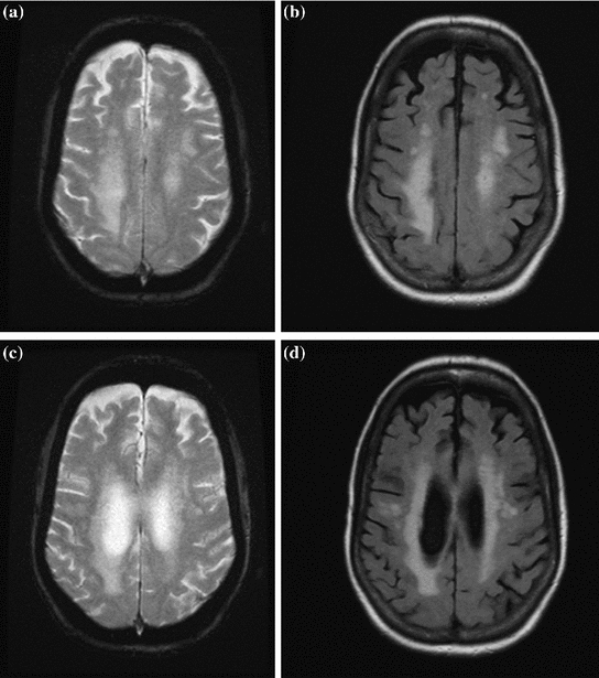


 . b
. b