coordinates for each point  [3]. Alternatively, a PDM can be built to examine the principal modes of point covariance [4]. Let
  denote a vector comprising 3D Euclidean coordinates of
  points sampled from the boundary of a brain structure. Assuming
  follows a multivariate normal distribution, parameterized by a mean point vector
  and a covariance matrix
  ,
,  can be decomposed as a linear combination of eigenvectors
  of
of  about
about :
:
(1)
 corresponds to the principle modes of variability and shape is represented by the set of scalar coefficients
  . One can thus examine the main shape variability by retaining a subset of
  ’s. We highlight that PDM is often used as constraints for segmentation. This approach is commonly referred to as the active shape model (ASM) [4] and can be augmented with appearance information [5].
The key challenge to point-based representations is that certain brain features may not be identifiable or may not even exist in all subjects. Manual means for correspondence creation by finding distinctive matching features, such as corners, are very time consuming. Automated methods, such as landmark detectors [6], provide a more repeatable means, but defining general features that are robust to inter-subject variability is non-trivial. In healthy, normal brains, the same brain structure may exhibit varying morphologies across subjects, e.g. due to different folding patterns associated with the same sulcus [7], and homologous features do not necessarily exist over the course of normal brain development, e.g. between gestational and infant stages. In the case of abnormality, pathology may be present or healthy tissue may be deformed or missing due to surgical resection.
2.1.2 Applications and Insights
The PDM has been used for aligning and segmenting subcortical structures such as the globus-pallildus, thalamus, caudate nucleus [8] and cortical structures such as sulci and gyri [9]. When using the traditional ASM, MR images must be aligned via similarity or affine transform to a common reference frame, since the model does not account for global variation in orientation. Further, homologous points along the boundary of structures to be segmented must be specified in a set of training images. A fundamental challenge is to define and identify homologous points on shapes with no distinct landmarks. This challenge may be potentially alleviated by using automatic tools for shape segmentation [10], landmark matching [11], and optimal point-based shape parameterizations, e.g. minimum description length [12]. However, inter-subject variability of the cortical surface render segmentation of cortical structures via PDM approaches non-trivial.
2.2 Local Feature-Based Approach
The idea behind local feature-based approach is to use intensity information to identify corresponding points across subjects, which can be viewed as a generalization of the traditional position-based models. A summary of commonly-used generic features is first provided, with a focus on the scale-invariant feature transform (SIFT), which has shown to be robust for many applications. Techniques for modeling brain shapes probabilistically with features extracted from training images are then described.
2.2.1 Feature Extraction
Feature-based shape modeling requires a means for robustly localizing distinctive image features reflective of the underlying brain anatomy. One approach is to construct specialized detectors to identify specific brain features, e.g. the longitudinal fissure [13], posterior tips of ventricles, etc. However, building specialized detectors for each brain structure can be quite labor demanding if whole-brain analysis is of interest. Towards this end, a number of generic feature detection methods has been proposed, which provides an automatic means for identifying distinctive features. Early methods in 2D image processing focused on finding salient patterns that can be reliably localized in the presence of arbitrary image translations and rotations, for instance, corner-like patterns that can be robustly extracted using spatial derivative operators [14]. This work was later extended to 3D volumetric brain images, which facilitates identification of a high number of generic brain landmarks [6].
A complication with spatial derivative operators is the choice of optimal spatial scale, which is typically unknown. Scale-space theory [15] formalizes the notion that landmark distinctiveness is intimately linked to the size or scale at which the image is observed. This led to the development of feature detectors designed to identify both the location and scale of distinctive image features, so-called scale-invariant feature detectors [16]. The field of image processing witnessed a number of scale-invariant feature detectors, primarily based on Gaussian derivatives in scale and in space, e.g. the SIFT method that identifies maxima in the difference-of-Gaussian (DoG) scale space [17]. SIFT has shown to provide robust matching features for brain analysis [18] in addition to various computer vision applications, and will be the focus for the remainder of this subsection.
A scale-invariant feature in 3D is a local coordinate reference frame consisting of a 3D point location  , a scale parameter
  , and an orientation matrix
  parameterized by orthonormal axis vectors
  . The local feature-based approach described here adopts the DoG operator in identifying feature points defined as
  of the DoG extrema:
  , where
  represents the convolution of an image with a Gaussian kernel of variance
  is the constant multiplicative sampling increment of scale, and
  denotes the set of all local maxima of
  . Although a variety of different saliency criteria could be adopted, the DoG criterion is attractive as it can be computed efficiently in
  time and memory complexity in the number of voxels N using scale-space pyramids [19].
, a scale parameter , and an orientation matrix parameterized by orthonormal axis vectors . The local feature-based approach described here adopts the DoG operator in identifying feature points defined as of the DoG extrema: , where represents the convolution of an image with a Gaussian kernel of variance is the constant multiplicative sampling increment of scale, and denotes the set of all local maxima of . Although a variety of different saliency criteria could be adopted, the DoG criterion is attractive as it can be computed efficiently in time and memory complexity in the number of voxels N using scale-space pyramids [19].To represent brain image features in a manner invariant to global image rotation, translation, and scaling, an important step is to assign a local orientation to the feature points. Local orientation information is particularly useful for alignment, which can be estimated via highly efficient algorithms, such as the Hough transform  time in the number of features N), to recover global similarity transforms and locally linear deformations [20]. The 3D orientation of a local feature point comprises three intrinsic parameters. These may be difficult to estimate unbiasedly due to the non-uniform joint density functions of common angular parameterizations, e.g. Euler angles, quaterions, etc. Instead, using feature-based alignment (FBA) [20] can be advantageous as it estimates direction cosine vectors of a
  rotation matrix
  from spherical gradient orientation histograms, which reduces the effect of parameterization bias.
time in the number of features N), to recover global similarity transforms and locally linear deformations [20]. The 3D orientation of a local feature point comprises three intrinsic parameters. These may be difficult to estimate unbiasedly due to the non-uniform joint density functions of common angular parameterizations, e.g. Euler angles, quaterions, etc. Instead, using feature-based alignment (FBA) [20] can be advantageous as it estimates direction cosine vectors of a rotation matrix from spherical gradient orientation histograms, which reduces the effect of parameterization bias.Once local orientation has been estimated, appearance features can be extracted from the image content within a local neighborhood of volume proportional to  around the point
  for establishing correspondence. Local appearance may simply be represented by raw image intensities [18], but the computer vision literature has demonstrated that alternative representations, such as the gradient orientation histogram (GoH), to be superior in terms of matching distinctiveness. The local feature-based approach adopts a variant of GoH by quantizing space and gradient orientation uniformly into an
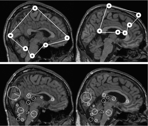
  element histogram. GoH elements are rank-ordered, where each element is assigned its rank in an array sorted according to bin counts, rather than the raw histogram bin count [21]. An example comparing PDM and local feature-based approach is shown in Fig. 1, in which PDM breaks down due to missing homologous brain features in the subjects [22].
around the point for establishing correspondence. Local appearance may simply be represented by raw image intensities [18], but the computer vision literature has demonstrated that alternative representations, such as the gradient orientation histogram (GoH), to be superior in terms of matching distinctiveness. The local feature-based approach adopts a variant of GoH by quantizing space and gradient orientation uniformly into an element histogram. GoH elements are rank-ordered, where each element is assigned its rank in an array sorted according to bin counts, rather than the raw histogram bin count [21]. An example comparing PDM and local feature-based approach is shown in Fig. 1, in which PDM breaks down due to missing homologous brain features in the subjects [22].Fig. 1
PDM versus local feature-based approach. Corresponding points extracted by PDM (upper pair) and local feature-based approach (lower pair) shown. PDM fails (upper right) due to unexpected inter-subject variability. The local feature-based model is stable, identifying robust scale-invariant feature correspondences (white circles) in cortical and sub-cortical regions
2.2.2 Probabilistic Modeling
Once scale-invariant features have been extracted from image data, they can be used as the basis for describing brain geometry and appearance probabilistically across a population. It is important to characterize variability within a normalized geometric frame of reference with variation in scale, rotation, and translation across different images removed. Let  represents a set of features extracted from an image, and let
  represent a global similarity transform that maps the image to a normalized reference frame.
  can be estimated using FBA [20], which employs a generative probabilistic model to learn the posterior probability of the unknown global similarity transform
  conditional on the feature data
  :
:
In this formulation,  is a latent random variable taking on discrete values
  with probability
  . Each value
  indicates a distinctive anatomical pattern, whose shape and appearance are encoded locally in normalized space by the density
  and by the occurrence probability
  . Note that the extracted features
  are conditionally independent given transform T, and that latent random variable f is independent of the transform T. The optimal alignment solution T* is taken as the one that maximizes the posterior probability (2). For the purpose of group analysis and classification, referred to as feature-based morphometry (FBM) [18], a random variable indicating subject group label
  is incorporated into the model. Subject group can be identified by maximizing the posterior probability of C conditional on the extracted features
  and T:
C is assumed to be independent of T and, as in the case of FBA, the extracted features  are assumed to be conditionally independent. Unlike FBA, latent feature shape and appearance densities
  and occurrence probability
  are conditioned on the group label in FBM, and can thus be used to identify group-informative structure and to quantify group differences. Classification and analysis can both be considered as identifying the group label C* that maximizes the Bayes decision ratio:
The decision ratio can be used to identify the optimal group label of a new subject. Note that the classification is heavily influenced by the product of likelihood ratios  associated with latent model feature
  . This likelihood ratio can be used to quantify the informativeness of the features with regard to group label, and can be used for identifying group-related anatomical structure.
represents a set of features extracted from an image, and let represent a global similarity transform that maps the image to a normalized reference frame. can be estimated using FBA [20], which employs a generative probabilistic model to learn the posterior probability of the unknown global similarity transform conditional on the feature data :(2)
is a latent random variable taking on discrete values with probability . Each value indicates a distinctive anatomical pattern, whose shape and appearance are encoded locally in normalized space by the density and by the occurrence probability . Note that the extracted features are conditionally independent given transform T, and that latent random variable f is independent of the transform T. The optimal alignment solution T* is taken as the one that maximizes the posterior probability (2). For the purpose of group analysis and classification, referred to as feature-based morphometry (FBM) [18], a random variable indicating subject group label is incorporated into the model. Subject group can be identified by maximizing the posterior probability of C conditional on the extracted features and T:(3)
are assumed to be conditionally independent. Unlike FBA, latent feature shape and appearance densities and occurrence probability are conditioned on the group label in FBM, and can thus be used to identify group-informative structure and to quantify group differences. Classification and analysis can both be considered as identifying the group label C* that maximizes the Bayes decision ratio:(4)
associated with latent model feature . This likelihood ratio can be used to quantify the informativeness of the features with regard to group label, and can be used for identifying group-related anatomical structure.The estimation of T* and C* require learning: the latent feature set  , probabilities
  and
and  , and likelihoods
  and
and  . Here,
  and
and  are assumed to be conditional Gaussian densities over the individual features
  parameterized by mean and variance vectors. Probabilities
  and
and  are parameterized by normalized feature occurrence counts. Computation of maximum likelihood estimates of the density and probability parameters can be posed as a clustering problem with cluster centers of the features extracted from training data that are similar in geometry and appearance being the estimates.
, probabilities and , and likelihoods and . Here, and are assumed to be conditional Gaussian densities over the individual features parameterized by mean and variance vectors. Probabilities and are parameterized by normalized feature occurrence counts. Computation of maximum likelihood estimates of the density and probability parameters can be posed as a clustering problem with cluster centers of the features extracted from training data that are similar in geometry and appearance being the estimates.With probability and density parameters estimated, T* and C* can be determined by computing their respective posterior probabilities based on nearest neighbor correspondences between extracted image and latent model feature appearance vectors. T* can thus be estimated in a manner similar to the Hough transform, and C* is estimated in a manner similar to a Naïve Bayes classifier. An example illustrating the application of the feature-based model for alignment and group analysis is shown in Fig. 2.
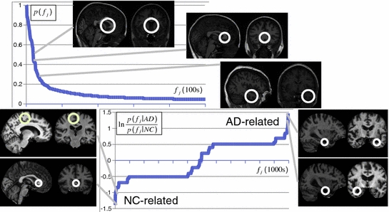
Fig. 2
Scale-invariant feature-based model for alignment and group analysis. Above Latent feature probability  can be used to identify stable neuroanatomical patterns across a population and quantify their occurrence frequency [20]. Below latent features can be related to subject group, such as normal control (NC) and Alzheimer’s disease (AD), by the likelihood ratio
  for identifying group-related neuroanatomical structure [18]
can be used to identify stable neuroanatomical patterns across a population and quantify their occurrence frequency [20]. Below latent features can be related to subject group, such as normal control (NC) and Alzheimer’s disease (AD), by the likelihood ratio for identifying group-related neuroanatomical structure [18]2.2.3 Applications and Insights
The local feature-based approach has a variety of possible applications. The first is as a means for achieving efficient, robust alignment of difficult brain image data even in the face of missing one-to-one homology. This task is a precursor to analyzing challenging data [20, 23]. The result of alignment is not only a global similarity transform  but also a set of probable image-to-model feature correspondences that quantify local residual geometrical variation. These correspondences have been shown to be effective in initializing deformable alignment of difficult data, e.g. enlarged ventricles in infant Krabbe disease [24]. Second, latent features from the trained model can be used to identify anatomical structure most representative of a population, or image structure most characteristic of specific groups. Further, this information permits prediction of group labels for new image data, e.g. in a computer-assisted diagnosis scenario [18] or to predict continuous variables, such as the age and possibly the developmental stage of the infant brain [25]. Lastly, the local feature-based approach is applicable for a variety of image modalities and can be adapted for inter-modality correspondence [23]. This approach lends itself to alignment and analysis algorithms that are highly efficient in terms of computation time and memory footprint, and is thus effective in modeling and analyzing brain structure in large image databases or across bandwidth-limited networks.
but also a set of probable image-to-model feature correspondences that quantify local residual geometrical variation. These correspondences have been shown to be effective in initializing deformable alignment of difficult data, e.g. enlarged ventricles in infant Krabbe disease [24]. Second, latent features from the trained model can be used to identify anatomical structure most representative of a population, or image structure most characteristic of specific groups. Further, this information permits prediction of group labels for new image data, e.g. in a computer-assisted diagnosis scenario [18] or to predict continuous variables, such as the age and possibly the developmental stage of the infant brain [25]. Lastly, the local feature-based approach is applicable for a variety of image modalities and can be adapted for inter-modality correspondence [23]. This approach lends itself to alignment and analysis algorithms that are highly efficient in terms of computation time and memory footprint, and is thus effective in modeling and analyzing brain structure in large image databases or across bandwidth-limited networks.3 Mesh-Based Representation: A Spectral Analysis Approach
The boundary between tissue types contains important information for characterizing brain shape. By representing this boundary as a surface, we can exploit powerful tools from intrinsic geometry. In this section, we review works that use the spectrum of surfaces for the intrinsic surface analysis, which has led to novel ways of surface reconstruction, classification, feature extraction, and computation of conformal maps.
3.1 Laplace-Beltrami Eigen-System
Let M denote a surface in  . Its Laplace-Beltrami (LB) eigen-system is defined as:
where  is the LB operator on M and f is a smooth function defined over M. Since the LB operator is self-adjoint, its spectrum is discrete and can be ordered by the magnitude of the eigen-values as
  If M is a surface with boundary, we can solve the eigen-system with the Neumann boundary condition. Some special examples of the LB eigen-system are widely used in signal processing. In the Euclidean domain, the LB eign-functions are the Fourier basis. On the unit sphere, the LB eigen-functions are spherical harmonics. Due to symmetry, the spherical harmonics have multiple eigen-functions for a single eigenvalue. For the
  th order spherical harmonics, there are
  eigen-functions. This multiplicity, however, is not general. For arbitrary surfaces without such symmetry, it was proved that this is not an issue [26].
. Its Laplace-Beltrami (LB) eigen-system is defined as:(5)
is the LB operator on M and f is a smooth function defined over M. Since the LB operator is self-adjoint, its spectrum is discrete and can be ordered by the magnitude of the eigen-values as If M is a surface with boundary, we can solve the eigen-system with the Neumann boundary condition. Some special examples of the LB eigen-system are widely used in signal processing. In the Euclidean domain, the LB eign-functions are the Fourier basis. On the unit sphere, the LB eigen-functions are spherical harmonics. Due to symmetry, the spherical harmonics have multiple eigen-functions for a single eigenvalue. For the th order spherical harmonics, there are eigen-functions. This multiplicity, however, is not general. For arbitrary surfaces without such symmetry, it was proved that this is not an issue [26].For numerical computation, a surface is often represented as triangular meshes created using the finite element method. Let  denote the triangular mesh representation of the surface, where V is the set of vertices and T is the set of triangles. Using the weak form of (5), we can compute the eigen-system by solving:

where the two matrices can be derived using the finite element method:
where  is the set of vertices in the 1-ring neighborhood of
  is the set of triangles sharing the edge
  is the angle in the triangle
  opposite to the edge
  , and Area
  is the area of the
  triangle
  .
.
denote the triangular mesh representation of the surface, where V is the set of vertices and T is the set of triangles. Using the weak form of (5), we can compute the eigen-system by solving:(6)
(7)
(8)
is the set of vertices in the 1-ring neighborhood of is the set of triangles sharing the edge is the angle in the triangle opposite to the edge , and Area is the area of the triangle .Fig. 3
LB eigen-functions on a hippocampal mesh model. i denotes the order of the eigen-function. a Mesh. b i = 1. c i = 25. d i = 50. e i = 100. With increasing order, the eigen-function becomes more oscillatory
As an illustration, the spectrum of a hippocampus is plotted in Fig. 3. We can see that the eigen-function becomes more oscillatory with increasing order. Thus, higher order LB eigen-functions can be considered as higher frequency basis, where frequency is intuitively the number of sign changes over the surface. This is reminiscent of the Fourier basis functions on Euclidean domain. This intuition is useful for signal processing applications on the surface. In [27], the LB eigen-functions were used for denoising signal defined on surface patches. For shape analysis, the LB basis functions were used to form a subspace for outlier detection and the generation of smooth mesh representation of anatomical boundaries [28]. For different surfaces, the number of nodal domains is also different and can be used as a signature for surface classification [29], which is similar to the shape DNA concept [30]. Next we present two different ways of using the LB eigen-functions to study brain surfaces.
3.2 Reeb Graph of LB Eigen-Functions
Many brain surfaces have obvious characteristics that are invariant to the orientation of the brain. For example, the hippocampus has the tail-to-head elongated trend. The cortical surface has the superior-to-inferior, frontal-to-posterior, and medial-to-later trend. The LB eigen-functions are very effective in capturing these global characteristics of brain surfaces. One powerful tool for this purpose is the Reeb graph of the LB eigen-functions, which can transform functions into explicit graph representations.
Given a function defined on a manifold, its Reeb graph [31] describes the neighboring relation between the level sets of the function. For a Morse function f on the mesh M, its Reeb graph is mathematically given by the following definition [31]:
Definition 1: Let  . The Reeb graph
  of f is the quotient space with its topology defined through the equivalent relation
  if
if  for
for  .
.
. The Reeb graph of f is the quotient space with its topology defined through the equivalent relation if for .As a quotient topological space derived from M, the connectivity of the elements in  , which are the level sets of f, change topology only at critical points of f. Reeb graph is essentially a graph of critical points. If f is a Morse function [32], which means the critical points of f are non-degenerative, the Reeb graph
  encodes the topology of M and it has g loops for a manifold of genus g. For a Morse function on a surface of genus-zero topology, its Reeb graph has a tree structure.
, which are the level sets of f, change topology only at critical points of f. Reeb graph is essentially a graph of critical points. If f is a Morse function [32], which means the critical points of f are non-degenerative, the Reeb graph encodes the topology of M and it has g loops for a manifold of genus g. For a Morse function on a surface of genus-zero topology, its Reeb graph has a tree structure.For the Reeb graph to be useful in medical shape analysis, it is critical to build it from a function reflective of the underlying geometry. The height function was a popular choice in previous work, such as surface reconstruction from contour lines [33] and the analysis of terrain imaging data [34, 35], but it suffers from the drawback of being pose dependent and thus not intrinsic to surface geometry. Functions derived from geodesic distances [36–39] were proposed to construct pose invariant Reeb graphs in computer graphics. However, geodesic distances are known for their non-robustness when topological changes are involved [40, 41].
Fig. 4
Reeb graph computation via sampling level contours. a Left eigen-functions. Right Reeb graph as skeleton. b Left eigen-functions. Right Reeb graph as medial cores
For the numerical construction of the Reeb graph, there are various approaches. Based on the intuition that Reeb graph encodes the relation of level sets on surfaces, we could simply sample a set of level contours on the surface and connect them using their neighboring relations. This approach is especially useful as a novel way of constructing skeleton or medial core of surfaces. Examples of level contours and the constructed Reeb graphs for the cingulate gyrus and hippocampus are shown in Fig. 4. For more complicated surfaces with large numbers of holes and handles, the sampling approach becomes computationally expensive because extremely dense sampling is needed to capture all the topological changes of level contours. To overcome this challenge, a novel algorithm is proposed in [42] that analyzes the topology of level contours in the neighborhood of critical points. As an illustration, the level contours in the neighborhood of a saddle point on a double torus are shown in Fig. 5b.
With increasing LB eigen-function, the level contour split into two contours. The mesh is then augmented such that the level contours become edges of the mesh. This makes it possible to use region growing on the augmented mesh to find branches of the Reeb graph. By scanning through all critical points (Fig. 5c), we can capture the topology of the level contours and build the Reeb graph (Fig. 5d). The surface partition generated by the Reeb graph ensures each surface patch is a manifold, so that further analysis of geometry and topology, such as the computation of geodesics, can be performed. For more details, see [42]. Since this method only needs to analyze the neighborhood of critical points, it can easily handle large meshes with hundreds of handles and holes. The Reeb graph provides a unified approach for topological and geometric analysis of surfaces. It has been successfully applied to develop a new way of topology and geometry correction in cortical surface reconstruction from MR images [42]. As an illustration, we show a cortical reconstruction example in Fig. 6a and c show the surface before and after correction from FreeSurfer [43]. Fig. 6b and d show the surface before and after correction generated by the Reeb analysis method. As highlighted in the circled region, clearly the latter generated better reconstruction.
Fig. 5
Reeb graph computation as graph of critical points. a Eigen-function on a surface. b Level contours in the neighborhood of a saddle point. c Reeb graph construction. d Surface partition with its Reeb graph
Fig. 6
Reeb analysis for unified corection of geometric and topological outliers in cortical surface reconstruction. a and c FreeSurfer reconstruction result before and after correction. b and d Reconstruction before and after Reeb-analysis based correction
3.3 LB Embedding Space
Using the LB eigen-system, we can build an embedding of the surface in the infinite dimensional  space that has the advantage of being isometry invariant. This allows intrinsic comparison of surfaces and leads to novel algorithms for surface maps.
space that has the advantage of being isometry invariant. This allows intrinsic comparison of surfaces and leads to novel algorithms for surface maps.Let  a set of eigen-functions. The embedding
  is defined as [40]:
For any two surfaces,  and
and  , rigorous distance measures between them can be defined in the embedding space, e.g. the spectral
  distance,
  [44]:
[44]:
where  and
and  are any given LB orthonormal basis of
  and
and  ,
,  and
and  denote the set of all possible LB basis on
  and
and  and
and  are normalized area elements, i.e.,
  and
and  . Using this distance, intrinsic matching of surfaces can be performed. For example, it has been successfully applied to surface classification and sulcal landmark detection [44]. One critical result of the spectral
  -distance is that it equals zero if and only if the two surfaces are isometric. This provides a new way of computing conformal surface maps, which are important tool for studying anatomical surfaces.
a set of eigen-functions. The embedding is defined as [40]:(9)
and , rigorous distance measures between them can be defined in the embedding space, e.g. the spectral distance, [44]:(10)
(11)
(12)
and are any given LB orthonormal basis of and , and denote the set of all possible LB basis on and and are normalized area elements, i.e., and . Using this distance, intrinsic matching of surfaces can be performed. For example, it has been successfully applied to surface classification and sulcal landmark detection [44]. One critical result of the spectral -distance is that it equals zero if and only if the two surfaces are isometric. This provides a new way of computing conformal surface maps, which are important tool for studying anatomical surfaces.Given two surfaces  and
and  , there exists a conformal metric
  , where
  is a positive function defined on
  , such that the LB embedding
  of
of  under this new metric will be the same as the LB embedding
  of
of  because the LB embedding is completely determined by the metric, where
  and
and  are the optimal basis that minimize the spectral
  distance. Since
  and
and  are conformal, and the two manifolds
  and
and  are isometric when the metric w is chosen so that the spectral
  distance is zero [44], we have a conformal map from
  to
to  when we combine these maps [45]. Let Id denote the identity map from
  to
to  , the conformal map
  is defined as:
![$$\begin{aligned} \mu (x)=\left[ {I_{M_2 }^{\Phi _2^*} } \right] ^{-1}\circ Id\circ I_{M_1 }^{\Phi _1^*} (x){\begin{array}{ll} &{} {\forall x\in M_1 } \\ \end{array} }, \end{aligned}$$](/wp-content/uploads/2016/10/A312883_1_En_1_Chapter_Equ13.gif)
To numerically compute the conformal map that minimizes the spectral -distance, a metric optimization approach was developed [45] that iteratively updates the weight function w to deform the embedding such that it matches that of the target surface. As an illustration, we show in Fig. 7 the conformal maps from a cortical surface to the unit sphere or a target cortical surface.
and , there exists a conformal metric , where is a positive function defined on , such that the LB embedding of under this new metric will be the same as the LB embedding of because the LB embedding is completely determined by the metric, where and are the optimal basis that minimize the spectral distance. Since and are conformal, and the two manifolds and are isometric when the metric w is chosen so that the spectral distance is zero [44], we have a conformal map from to when we combine these maps [45]. Let Id denote the identity map from to , the conformal map is defined as:(13)
Fig. 7
A comparison of conformal maps. a Source surface  . b Conformal map to the unit sphere. c Metric distortion from
  to the sphere. d Conformal map from
  to a target cortical surface
  . e Metric distortion from
  to
to 
. b Conformal map to the unit sphere. c Metric distortion from to the sphere. d Conformal map from to a target cortical surface . e Metric distortion from to The source surface shown in Fig. 7a is colored with its mean curvature. The conformal map to the unit sphere, shown in Fig. 7b, is computed with the approach in [46] that minimizes the harmonic energy. The conformal map to the target cortical surface, shown in Fig. 7d, is computed with the metric optimization approach that minimizes the spectral  -distance in the embedding space. The mean curvature on the source surface is projected onto the sphere and target surface using the maps. We can see large distortions of triangles in the spherical map. On the other hand, the gyral folding pattern is very well matched in the map to the target cortical surface. From the histogram plotted in Fig. 7c and e, we can see metric is much better preserved in the conformal map computed with the metric optimization approach.
-distance in the embedding space. The mean curvature on the source surface is projected onto the sphere and target surface using the maps. We can see large distortions of triangles in the spherical map. On the other hand, the gyral folding pattern is very well matched in the map to the target cortical surface. From the histogram plotted in Fig. 7c and e, we can see metric is much better preserved in the conformal map computed with the metric optimization approach.Since the metric optimization approach can produce maps that align major gyral folding patterns of different cortical surfaces, a multi-atlas fusion approach has been developed to automatically parcellate the cortical surface into a set of gyral regions [45]. With metric optimization, a group-wise atlas is first computed in the embedding space. The conformal map from each atlas to the group-wise atlas is then computed. Using the property that the composition of conformal maps is still conformal, only one map to the group-wise atlas needs to be computed for an unlabeled surface. With maps to all the labeled atlases, a fusion approach can be developed to derive the labels on new surfaces. As a demonstration, we plotted in Fig. 8 the labeling results on the left and right hemispherical surfaces of two subjects. We can clearly see that excellent labeling performances have been achieved.
Fig. 8
Automatic labeling of cortical gyral regions
3.4 Application and Insights
The spectral analysis approach provides a general and intrinsic way of studying anatomical shapes. The LB embeddings and features derived from the spectral analysis have the advantage of being isometry invariant, which makes them robust to deformations due to variability across populations, normal development, and pathology. The mathematical foundation of the spectral analysis is applicable to shapes of arbitrary dimension and topology. With little adaptation, the spectral analysis techniques can be easily applied to many different anatomical shapes. It has been applied for mapping subcortical structures in brain mapping studies [47] and automated labeling of complicated cortical surfaces [45]. The Reeb graphs constructed from the eigen-functions could also be a general tool for topology analysis in medical imaging.
4 Function Representation
Brain shape can be described implicitly using various classes of functions, computed over the normalized image domain, i.e. images normalized with respect to similarity transform. This section discusses several methods by which this can be done: moment invariants, the distance transform, and linear projections: global and local frequency decompositions over Euclidean and spherical coordinates.
4.1 Moment Invariants
Let  be an image indexed by coordinates
  . Geometrical moments are defined as expectations computed across the image:
Moments can be referred to by their order  , and are useful in shape description as they have intuitive geometrical interpretations. For instance, the
  order raw moment
  represents the sum of image intensities or shape volume. The
  order raw moments
  normalized by
  are the centers of mass of a shape:
  . A key aspect of moments is that they can describe shape in a manner invariant to classes of image transforms that are irrelevant to shape description, e.g. similarity transform. Invariance to translation can be achieved by computing central moments about the center of mass:
Invariance to scale changes is achieved by normalizing central moments by a suitable power of the  th order moment:
The  nd order central moments correspond to spatial variance of an intensity pattern in 3D space, and
  rd order central moments provide a measure of skew. Moments are not generally invariant to rotation, but such invariance can be achieved by combining the moments in certain ways [48, 49]. A number of additional aspects of moments bear mentioning. Moments can generally be used to reconstruct the original image. Moments are related to global shape characteristics, and thus not be suitable for identifying local variations. A variety of moments exist other than geometrical moments, including Zernike moments, Legendre moments, and rotational moments.
be an image indexed by coordinates . Geometrical moments are defined as expectations computed across the image:(14)
, and are useful in shape description as they have intuitive geometrical interpretations. For instance, the order raw moment represents the sum of image intensities or shape volume. The order raw moments normalized by are the centers of mass of a shape: . A key aspect of moments is that they can describe shape in a manner invariant to classes of image transforms that are irrelevant to shape description, e.g. similarity transform. Invariance to translation can be achieved by computing central moments about the center of mass:(15)
th order moment:(16)
nd order central moments correspond to spatial variance of an intensity pattern in 3D space, and rd order central moments provide a measure of skew. Moments are not generally invariant to rotation, but such invariance can be achieved by combining the moments in certain ways [48, 49]. A number of additional aspects of moments bear mentioning. Moments can generally be used to reconstruct the original image. Moments are related to global shape characteristics, and thus not be suitable for identifying local variations. A variety of moments exist other than geometrical moments, including Zernike moments, Legendre moments, and rotational moments.4.2 Distance Transform
Let S be the set of all point locations along the boundary of a segmented brain structure. The distance transform of a shape S is an image  , where the value at location
  reflects the distance
  between
  and the closest location
  :
:
There are a number of commonly-used distance functions, such as Euclidean distance and Manhattan distance. Figure 9 shows the Euclidean distance transform for a cross section of the corpus callosum. The distance transform can be considered as a local shape description, as the value of  is determined by the nearest boundary point in S. The value
  can be interpreted as the radius of the largest sphere about point
  lying within the boundary S. The set of ridges in
  can be used for extracting medial axes as to be discussed in Sect. 5.
, where the value at location reflects the distance between and the closest location :(17)
is determined by the nearest boundary point in S. The value can be interpreted as the radius of the largest sphere about point lying within the boundary S. The set of ridges in can be used for extracting medial axes as to be discussed in Sect. 5.Fig. 9
Distance transform of corpus callosum
4.3 Frequency Decomposition
Shape in an image  can be represented implicitly by projection onto an orthogonal basis with the Fourier basis being arguably the most widely-used. Let
  be a discrete image of size
  . The discrete Fourier transform (DFT)
  of an image is obtained by projection onto an orthonormal complex exponential basis:
The DFT has several properties that are of interest for shape representation. In particular, the magnitude of the power spectrum is invariant to translation and a significant portion of shape related information is embedded in the phase portion of the signal. Further, the DFT can be inverted to reconstruct the original image:
The DFT can be computed efficiently in  in the number of samples N using the fast Fourier transform (FFT) algorithm. The convolution theorem can be used to implement linear filtering operations efficiently in
  time complexity in the Fourier domain. For natural objects, such as the brain, the power of the Fourier spectrum is concentrated in low frequency components, i.e. small values of
  , which arise from large-scale spatial structure.
can be represented implicitly by projection onto an orthogonal basis with the Fourier basis being arguably the most widely-used. Let be a discrete image of size . The discrete Fourier transform (DFT) of an image is obtained by projection onto an orthonormal complex exponential basis:(18)
(19)
in the number of samples N using the fast Fourier transform (FFT) algorithm. The convolution theorem can be used to implement linear filtering operations efficiently in time complexity in the Fourier domain. For natural objects, such as the brain, the power of the Fourier spectrum is concentrated in low frequency components, i.e. small values of , which arise from large-scale spatial structure.The classical DFT operating on Cartesian image data is rarely used to characterize shape in the brain directly, as neuroanatomical structures are often represented in terms of a spherical topology. For example, the cortex is often inflated or flattened onto a sphere index by [50], and structures, such as the putamen, can be represented as a simply connected 3D surfaces [51]. Spherical harmonics (SH) generalize frequency decompositions to functions on the sphere. Let  represent a function on the unit sphere parameterized in angular coordinates
  . The spherical harmonic representation is expressed as:
where shape is represented by harmonic coefficients  in a manner analogous to Fourier coefficients. The basis
  is given by:
where  is the Legendre polynomial of degree l and order m, and
  is a normalization factor. Although rotation dependent, coefficients
  can be used to compute rotation invariant shape descriptors [46]. Efficient computation of spherical harmonic coefficients is possible via fast discrete Legendre transform [52].
represent a function on the unit sphere parameterized in angular coordinates . The spherical harmonic representation is expressed as:(20)
in a manner analogous to Fourier coefficients. The basis is given by:(21)
is the Legendre polynomial of degree l and order m, and is a normalization factor. Although rotation dependent, coefficients can be used to compute rotation invariant shape descriptors [46]. Efficient computation of spherical harmonic coefficients is possible via fast discrete Legendre transform [52].4.4 Local Frequency Decomposition
The aforementioned frequency decompositions are useful as global descriptors of brain structures. However, they are not suited for localizing specific areas of variability, e.g. a small fold on a surface. A collection of function-based techniques have been developed to characterize image shape locally. For encoding and reconstruction, an image may be projected onto a wavelet basis [53], consisting of translated and scaled versions of a mother wavelet function  :
:
where  are 3D translation and scaling parameters. Shape is captured by wavelet coefficients
  , where a significantly non-zero coefficient
  indicates the presence of a local feature within a region of size
  about the image location
  . An important aspect of wavelet analysis is the design or choice of the mother wavelet function. The choice typically depends on the requirements of the image analysis task at hand, e.g. for compression and reconstruction, complete orthonormal basis is often used. However, complete wavelet basis may be overly sensitive, i.e. minor translations or scaling could result in dramatic changes in wavelet coefficients. Scale-space theory [54] shows that the Gaussian kernel is optimal for multi-scale image representation with respect to an intuitive set of axioms including translation and shift invariance, rotational symmetry, and non-creation or enhancement of local extrema. The Gaussian scale space can be considered as an overcomplete wavelet representation.
:(22)
are 3D translation and scaling parameters. Shape is captured by wavelet coefficients , where a significantly non-zero coefficient indicates the presence of a local feature within a region of size about the image location . An important aspect of wavelet analysis is the design or choice of the mother wavelet function. The choice typically depends on the requirements of the image analysis task at hand, e.g. for compression and reconstruction, complete orthonormal basis is often used. However, complete wavelet basis may be overly sensitive, i.e. minor translations or scaling could result in dramatic changes in wavelet coefficients. Scale-space theory [54] shows that the Gaussian kernel is optimal for multi-scale image representation with respect to an intuitive set of axioms including translation and shift invariance, rotational symmetry, and non-creation or enhancement of local extrema. The Gaussian scale space can be considered as an overcomplete wavelet representation.As in the case of global frequency representation, a significant research focus has been to translate local frequency decompositions from Euclidean space to the spherical topology as commonly used in brain shape analysis. Yu et al. proposed an approach whereby wavelet coefficients are computed from the cortical surface mapped to the unit sphere by successively subdividing an icosahedron tilling [55]. Bernal-Rusiel et al. [56] compared smoothing using Gaussian and spherical wavelet techniques, finding that spherical wavelet smoothing may be better suited for preserving cortical structure in the case of spherical cortex data. Kim et al. [57] demonstrated that the wavelet transform can be generalized to an arbitrary graph over the cortical surface, which avoids sampling issues when mapping the cortical surface to a sphere.
4.5 Applications and Insights
In the seminal work of Hu [48], moment invariants were used to describe the shape of 2D image patterns. This was subsequently generalized to 3D volumetric data [49, 58]. In brain shape analysis, moment invariants have been used to describe the shape of cortical gyri [59] and regional activation patterns in functional MRI studies [60]. Principal component analysis of 2nd order moments has also been explored for describing and assigning an orientation axis to shapes, such as gyri [61]. Further, moment invariants have been employed in the context of abnormal shape variations, for instance, as a basis for image registration [62] or to identify aneurisms [63].
The distance transform has been used in segmenting brain structures, such as the corpus callosum and abnormal structure, such as tumors [64]. Also, distance transform is often used for initialization and evolution of contour-type segmentation algorithms, such as level sets. The distance transform can also be used as the basis for registration, as it remains unchanged under image translation and rotation [65].
Related posts:
Stay updated, free articles. Join our Telegram channel

Full access? Get Clinical Tree


