6 Ultrasound Imaging
Introduction
An ultrasound image is formed using sound. Ultrasound has been widely used because it is portable, low cost, and does not involve ionizing radiation; thus, it is safe even for scanning a fetus. B-mode ultrasound image formation is based upon three basic assumptions:1
The sound travels in a straight and narrow line called an acoustic beam. A transducer is used both as a pulse emitter and as an echo receiver. The transducer emits a short pulse and then receives echo signals which are generated by the emitted pulse propagating and interacting with tissue within the acoustic beam.
The speed of the sound propagation is assumed to be constant at 1,540 m/s, an average speed for soft tissues. Therefore, on the image, the sources for echo signals are localized by the so-called range equation:

Where t is the time delay between the pulse emission and the echo reception, c represents the speed of sound (i.e., 1,540 m/s is assumed for soft tissue), and D is the depth of the echo where it is generated. The time delay t includes both the time it takes for the pulse to travel down to the reflector and the time it takes for the echo to return. Therefore, it accounts for the factor of 2.
The received echo signals are amplified to compensate for the attenuation. The strength of the echo signals is represented by varying brightness levels on a B-mode image.
Ultrasound images are formed using the idealized model described above. Ultrasound artifacts occur when any or all of the assumptions are violated.
Common Image Quality Problems
Speed of sound propagation: it affects spatial resolution and the accuracy of the distance measurements.
Frequency: it affects spatial resolution and the maximum depth of penetration.
Array transducer dropouts: the deficiency most commonly found during routine quality control (QC) testing.
Presets in image protocols: optimize the image acquisition controls and maintain the consistency by managing the “presets” in image protocols.
Acoustic window: it affects the coupling of the transducer and patient body. A poor acoustic window prevents the sound from being transmitted to the region of interest.
Reverberation artifacts such as comet-tail and ring-down can provide diagnostic information.
Range ambiguity occurs when the pulse repetition frequency (PRF) is too high with the result that echoes from the prior beam line are mispositioned in the current beam line.
Enhancement and shadowing can provide diagnostic information.
Harmonic imaging is advantageous over conventional B-mode imaging in generating superior image quality, especially in the case of a “technically difficult” patient with a thick body wall.
The performance evaluation of the ultrasound scanner display and the reading room workstation displays is crucial in maintaining consistency of image perception.
Doppler aliasing occurs when the PRF is too low, a control that is linked to the PRF. To reduce aliasing, one should increase the velocity scale.
6.1 Case 1: Pulse-Echo Imaging Principle and Speed of Sound Propagation
6.1.1 Background
Size measurement is a routine clinical application in ultrasound imaging. The range equation is implicitly built into pulse-echo imaging instruments to localize the received echo signals. If the sound propagation speed in the body tissue is indeed 1540 m/s, the measured size will be accurate. However, if the sound propagation speed is less than 1540 m/s, then the longer delay in echo return time is interpreted by longer distance; in this case the distance in the axial direction is overestimated. On the other hand, if the speed is greater than 1540 m/s, then the distance in the axial direction is underestimated.
The misestimated sound propagation speed not only affects the distance measurement, but also contributes to the reduction of the spatial resolution; thus, it worsens the image quality.
6.1.2 Findings
In the following clinical case, the discontinuity seen in the diaphragm pointed by the arrow in Fig. 6‑1 a is caused by the different sound speed in the lesion. The sound speed reduces in a fatty lesion. Therefore, the portion of the diaphragm (pointed by the arrow) below the lesion is shown in a deeper position in the image. In another clinical case shown in Fig. 6‑1 b, an irregular liver/diaphragm interface is seen in the image caused by heterogeneous liver parenchyma with fatty infiltration.

The misestimated speed of sound propagation affects the image quality as demonstrated by the group of pins in Fig. 6‑2.

6.1.3 Discussion
The speed of sound propagation is dependent upon the tissue properties such as density and compressibility. For any particular material, the higher its density and the harder it is to compress, the faster its sound speed will be. For example, the sound speed is faster in bone than that in soft tissue because bone is more dense and harder to compress than soft tissue. Table 6‑1 shows the typical speed of sound propagation in a variety of materials. In diagnostic ultrasound, a sound speed of 1,540 m/s is assumed. This value represents the average speed of sound propagation in soft tissues. Any deviation from the assumed speed causes errors in size measurements, known as speed artifacts. As the acoustic beam focusing relies on the assumption of the sound speed, image quality is affected by any deviation in the actual sound speed and the assumed sound speed by the ultrasound system in setting up the beam former. As demonstrated in Fig. 6‑2, the beam focuses the best when the assumed sound speed matches the actual sound speed at 1460 m/s.
6.1.4 Resolution
It is important to recognize potential speed artifacts by examining the acoustic pathway and identifying regions that are suspected to have different values for sound speed. Typically, nothing is done to correct for speed artifacts. However, some modern ultrasound systems allow manual adjustment to correct for deviations in the speed of sound in order to improve image quality. As demonstrated in Fig. 6‑2, the actual speed of sound of the urethane-based phantom is approximately 6% lower than 1,540 m/s. 3 When the machine-assumed speed of sound does not match the actual speed of sound in the urethane-based phantom, the lateral resolution deteriorates. This feature has been used for breast imaging. As shown in Fig. 6‑3, the image quality is improved by an adjustment from the typical sound speed, i.e., 1,540 m/s to the actual sound speed in breast tissue at 1,500 m/s.

6.2 Case 2: Array Transducers and Sound Frequency
6.2.1 Background
Sound frequency is the number of oscillations per unit time, determined by the source—ultrasound transducer. For human ears, the audible sound frequency ranges from 20 Hz to 20 kHz. Sound with frequencies above 20 kHz is called ultrasound. The higher the frequency, the better the spatial resolution in ultrasound images. On the other hand, the lower the frequency, the deeper the ultrasound penetrates because the ultrasound attenuation is proportional to frequency. In medical ultrasound imaging, the frequency typically ranges from 2 to 15 MHz with low frequency used for imaging deep targets but with compromised spatial resolution, and high frequency used for imaging superficial targets with better spatial resolution. High frequencies, around 50 MHz or even higher, are used for certain specialized imaging applications, such as in ophthalmology or in small animal imaging, with superb spatial resolution.
An ultrasound system typically has multiple transducers of various frequencies, each transducer having a different contact surface size (footprint) designed for specific clinical applications. Modern ultrasound systems often allow the operator to choose the frequency within a range on the same transducer, which allows for adjustment between penetration and spatial resolution.
6.2.2 Findings
Different types of array transducers and their corresponding image examples are shown in ; Fig. 6‑4.

Linear Array
A subgroup of elements is fired to form one acoustic beam perpendicular to the face of the array.
Subgroups of elements are fired sequentially to form parallel acoustic beams to scan across a region of interest (ROI).
Rectangular shape of the image format.
Clinical applications include small parts, vascular, and obstetric exams (Fig. 6‑4a).
Curvilinear or Curved Array
Same as linear arrays except that the elements are aligned in a curve instead of a straight line.
Each acoustic beam is perpendicular to the face of the array. Since the array of elements is curved, the acoustic beams diverge with depth which allows for a broader coverage as the depth increases.
Clinical applications include general abdominal, obstetric, and transabdominal pelvic exams. In addition, transvaginal and transrectal probes are curved arrays (Fig. 6‑4b).
Phased Array
All the elements are fired to form one acoustic beam.
The acoustic beam is electronically steered across the ROI.
The footprint is typically very small to allow for a small acoustic window (e.g., between the ribs) but the sector image format allows for a broad field of view.
Clinical applications include intercostal scanning for heart, liver, or spleen (Fig. 6‑4c).
6.2.3 Discussion
On modern ultrasound systems, frequency can be selected within a certain range on the same transducer. While making the frequency selection, one must consider the fundamental trade-off between spatial resolution and penetration, and strike an optimal balance between these two factors (Fig. 6‑5).

6.2.4 Resolution
It is possible to improve penetration at high frequency with advanced technology such as coded excitation technology. This technology plants a code in the transmitted pulses. In return, the received echo signals are carrying the same code; thus, raising the ability to differentiate between echo signals and noises. Through appropriate coding on transmitted pulses and decoding on received echo signals, one can improve the signal-to-noise ratio and can, therefore, mitigate the trade-off between better spatial resolution, which is associated with higher frequency, and less penetration, also associated with higher frequency.
6.3 Case 3: Nonuniformity (Array Transducer Element Dropouts)
6.3.1 Background
An ultrasound array transducer contains an array (or arrays) of composite ceramic piezoelectric elements connected by wires enclosed in a cable that runs to the ultrasound system via a connector. An ultrasound transducer is vulnerable to damage because it is handled frequently during ultrasound imaging operation and may easily be dropped or bumped against hard surfaces, or its cable may be rolled underneath the scanner wheels during transportation for portable studies. An ultrasound transducer is prone to image nonuniformity problems due to any of the following defects: (1) failed crystal elements; (2) delamination of the lens/coupling layers on the transducer face; (3) broken wires in the transducer cable; and (4) disruptions in the connector. A picture of transducers with tangled cables connected to an ultrasound system is shown in Fig. 6‑6 a. Transducers are often hung on walls, as shown in Fig. 6‑6 b, c. Too much stress on a transducer cable may tear the wires inside the cable and cause element dropouts. Handling transducers with care is critical to ensuring the longevity of these array transducers.

6.3.2 Findings
Sometimes the nonuniformities are minor, appearing as streaks along the axial direction of the transducer, whereas some are more prominent. Fig. 6‑7 shows the images generated by the same transducer. Nonuniformities can be seen on the clinical image and the phantom image, as well as on the in-air scan image.

6.3.3 Discussion
Image nonuniformity is considered the most commonly found deficiency during routine QC testing.4 As shown in the example in Fig. 6‑8, the transducer cable was accidentally rolled underneath the scanner wheel and five wires in the cable were broken causing minor dark streaks near the face of the transducer. The broken wires were detected by an electronic transducer testing device.5 The nonuniformity was much less perceivable on clinical images.

6.3.4 Resolution
It is important to perform periodic QC testing using an ultrasound QC phantom to detect the presence of any nonuniformities as early as possible in order to monitor the condition and address the problem before clinical applications are impacted. The image uniformity test is a required QC test by American College of Radiology (ACR) Ultrasound Accreditation Program for all transducers used for clinical applications.6
Related posts:


Stay updated, free articles. Join our Telegram channel

Full access? Get Clinical Tree


