A Gamma Mixture Model for IVUS Imaging

Fig. 13.1

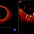
IVUS image in polar coordinates (a) and Cartesian coordinates (b) with the presence of lipidic (LIP) and calcified (CAL) plaques that were histologically identified

The acoustic response of different kinds of plaque is qualitative known: lipidic plaque presents low echolucent response; fibrous plaque presents intermediate level echogenicity; calcified plaque is hyperechogenic and usually presents an acoustic shadow due to the series of echoes created by multiple reflections within a small but highly reflective tissue [2–5].

However, although this qualitative characterization of the plaques offers an intuitive interpretation of IVUS images, an important effort has been done to understand the echo-morphology and pathological evolution [6]. A quantitative characterization of plaques allows developing or refining methods for plaque detection, risk predictions, and potentially suggesting different therapies.

Obtaining a quantitative characterization of the ultrasonic responses of plaques involve the analysis of the physics of ultrasound imaging throughout the acquisition process.

Basically, the process of image formation in medical ultrasound begins with the propagation of a pulse packet emission along the beam vector axis. This pulse changes its shape according to media properties The traveling pulse is scattered by objects placed at different scattering depths and cause delays in the pulse.

As a result, the backscattered (received) signal is corrupted by a characteristic granular pattern noise called speckle which depends on the number of scatterers per resolution cell as well as their size [7, 8]. This type of multiplicative noise, in the sense its variance depends on the underlying signal, is observed in other modalities using coherent radiation such as LASER [9] and Synthetic-Aperture Radar (SAR) [10].

Speckle mainly depends on the microstructure of the tissues and thus its statistics can be used as tissue histological descriptors [11]. These statistics strongly depend on the scatter density, that is, on the number and intensity distribution of the scatters in each resolution cell and the resulting speckle noise can be grouped in the following main classes:

Fully developed: large number of scatters (central limit theorem can be applied) per resolution cell and nonexistence of deterministic component, modeled by Rayleigh distribution [12, 13].
Fully resolved: large number of scatters per resolution cell and existence of deterministic component, modeled by Rice distribution [14].
Partially developed: small number of scatters per resolution cell and nonexistence of deterministic component, modeled by K distribution [15, 16].
Partially resolved: small number of scatters per resolution cell and existence of deterministic component, modeled by K-Homodyne distribution [17].

Fully developed speckle is the most common model for speckle formation. It considers a tissue or region composed of a large number of scatterers, acting as echo diffusers. These scatterers arise from inhomogeneity and structures approximately equal to or smaller in size than the wavelength of the ultrasound, such as tissue parenchyma, where there are changes in acoustic impedance on a microscopic level within the tissue.

There are different approximations for this model, the one-parameter probabilistic model that describe the pixel intensities in envelope data is by Rayleigh probability density function (PDF) [7, 13, 18].

Other distributions have been proposed for the characterization of speckle. Probably, the most noticeable distribution is the Nakagami proposed in [19]. This distribution has two parameters and can be considered as a generalization of the Rayleigh distribution. In [20], a model based on Nakagami distributions is proposed for the characterization of backscattered echo. This model is motivated from the fact that the Nakagami distribution generalizes the Rayleigh distribution and also appears to be similar to Rician distribution, which is also a generalization of the Rayleigh (see [20]).

Plaque echo-morphology is the contribution result of different tissue types (components). The lipidic plaque usually presents a fibrotic cap which has different acoustic response and thus different distributions [2]. Additionally, accumulation of blood cells (macrophages) within plaques may change their probabilistic models. Hence, a mixture model becomes an opportune strategy for statistically describing the echo-morphology of the plaque.

The Rayleigh mixture model (RMM) was first proposed in [8, 21] for plaque characterization and classification. In that work, a RMM was obtained by Expectation–Maximization method [22, 23]. Three kinds of plaque were considered in that study: fibrotic, lipidic, and calcified. The RMM parameters were estimated for each kind of plaque and were used, in combination to other textural features, to provide a descriptor of plaque composition. On the other hand, a Nakagami mixture model (NMM) was proposed in [24] for segmentation of arteries. This approach uses the Nakagami as a generalization of Rayleigh distribution as a good candidate to characterize the speckle.

Although the characterization of speckle can be modeled by different PDFs, the echo-morphology of plaque presents a more complicated nature than an isolated kind of speckle. It is the contribution result of different tissue types (components): the lipidic plaque usually presents a fibrotic cap which has different acoustic response and thus different distribution [2]. Additionally, the presence of macrophages within plaques change their probabilistic models.

The complexity of the composition of the plaque introduce difficulties when the echolucent response is modeled by a simple model such as a unimodal PDF (Rayleigh, Rice, K or K-Homodyne). Instead of that, a mixture model offers a good strategy for statistically describing the echo-morphology of the plaque. Among mixture models proposed in the literature for describing plaque characterization, two are of capital importance. On the one hand, a RMM which was first proposed in [8, 21] for plaque characterization and classification. In that work, a RMM was obtained by Expectation–Maximization method [22, 23]. Three kinds of plaque were considered in that study: fibrotic, lipidic, and calcified. The RMM parameters were estimated for each kind of plaque and were used, in combination to other textural features, to provide a descriptor of plaque composition.

On the other hand, a NMM was proposed in [24] for segmentation of arteries. This approach uses the Nakagami as a generalization of Rayleigh distribution as a good candidate to characterize the speckle. Note that both mixture models describe the behavior of speckle in the case of fully formed speckle. And the NMM could be considered as a generalization of the RMM.

Both the Rayleigh and the Nakagami have been commonly accepted assumptions for fully developed speckle. The former is justified because it is based on the physics of the data generation process, the later has proven to provide a better description since it is a two-parameter generalization of the Rayleigh. However, real-life cases of ultrasound images have shown that Rayleigh or Nakagami models do not describe it as good as expected. In [18, 25], many distributions were empirically fitted to real data and showed that fully developed speckle is better described by the Gamma distribution. Those distributions were tested in the resulting image after the reconstruction process, so it is clear that the different reconstruction stages modify dramatically the statistical behavior. This result was also confirmed in [7] where the PDFs were tested after the interpolation stage when no logarithmic compression is performed. In that work, experimental tests showed the superiority of the Gamma distribution over the Rayleigh and Nakagami for describing US data—85 % of the fully developed speckle areas passed the χ ² test when a Gamma distribution was fitted, whereas 70 % and less than 10 % passed in the Nakagami and Rayleigh cases respectively.

The interpolation operation performed in the A-lines of the raw RF signal to resample the data and equalize the resolution in both dimensions, angle and depth seems to be the key element to explain why Gamma describes better the data than the Rayleigh or Nakagami distributions. The interpolation process can be formulated as linear filter that linearly combines different pixels that are Rayleigh distributed. As shown in [7], a linear combination of Rayleigh random variables can be accurately fitted by Gamma distributions even when the central limit theorem can be applied (when the number of combinations of Rayleigh distributions is high enough to apply the central limit theorem). Note that the interpolation process consists of a weighted sum of values that, in the case of Rayleigh distributed data, results in a different random variable. Hence, not only interpolation processes but every linear filter applied to a Rayleigh distributed data is a weighted sum of Rayleigh random variables, which is better described by a Gamma random variable than a Rayleigh.

A common stage of the acquisition process of US images is to downsample the acquisition in order to provide an isotropic resolution of the image. This resampling stage usually involves an interpolation stage where linear filtering is applied. This interpolation is performed when the final resolution is not a multiple of the initial resolution. In these conditions, the results obtained in [7, 18, 25] still hold and the Gamma distribution better describe US RF envelope downsampled data than the Rayleigh or Nakagami distributions.

In this chapter we propose a Gamma mixture model (GMM) to describe the interpolated/resampled RF envelope US data. This model is compared with the other mixture models (Rayleigh and Nakagami) for different sort of plaques.

The characterization method provides probability maps which can be of help for physicians or for automatic postprocessing techniques such as filtering or segmenting methods. Concretely, a filtering method based on the estimation of the underlying parameters of the speckle is presented.

The rest of the chapter is structured as follows: in Sect. 2 we justify the better behavior of the Gamma PDF when linear filters and/or interpolation are applied. This justification follows that one presented in [7]. In Sect. 3 we describe the dataset, the acquisition protocols, and histological validation for plaques for which the comparison between methods is performed. Section 5 is devoted to the GMM, where the GMM is derived. The comparison between mixture models and experiments are presented in Sect. 6. As an application of the characterization of the GMM probability maps, a filter is proposed in Sect. 7. Finally, we conclude in Sect. 8.

2 Interpolation on Probabilistic Models for Ultrasonic Images

2.1 Overview

Some image filtering and segmentation techniques for ultrasound imaging, as those approaches based on maximum likelihood and maximum a posteriori [25], rely on an accurate statistical model for the different regions in the image. This model is usually derived from the analysis of the acoustic physics and the information available of the ultrasound probe [7, 26]. However, the whole information during the acquisition process is not usually available, and therefore some suppositions must be considered. For example, images provided by practitioners usually do not include the acquisition parameters as gain and/or contrast adjustment. Additionally, some of the steps of the acquisition process may be unknown, depending on the commercial firm of the ultrasound equipment.

In this section we focus on fully formed speckle. In fully formed speckle regions, acquired signal can be modeled following a Rayleigh distribution [13]. However, to form the final Cartesian image, these Rayleigh distributed data have to be interpolated. Thus, the resulting image will no longer follow a Rayleigh distribution. This section is devoted to model this final distribution taking into account the interpolation process [7, 26].

If no compression of the data is done (which will be an assumption throughout the section), we show that the results provided in literature [18, 25] hold with the interpolation probabilistic model here presented and that this approach can be extended easily to other distributions.

2.2 Interpolation Model

Ultrasonic images are constructed from a number of acoustic “lines” or vectors usually organized in a sequential pattern [26]. These vectors form lines in the image after conversion by envelope detection. Each line represents a time record of the scattered waves from different depths. The process of image formation begins with a pulse packet emission which travels along the beam vector axis and changes shape according to characteristics of the media. The traveling pulse is scattered by objects placed at different scattering depths and cause delays in the pulse. Reflections are received by the transducer and, considering a constant sound speed, the depths of the scattering objects can be estimated. These intercepted waves are integrated over the surface of the transducer with a suitable weighting and time delays are added for focusing and beamforming. The amplitude of the envelope record is usually logarithmically compressed but this is optional depending on the ultrasonic machine. At this point, when fully formed speckle regions are observed, a Rayleigh probabilistic distribution is often considered [9]. After this step all the lines are interpolated to form a complete Cartesian image from a number of image lines arranged in their geometrical attitude [7, 26].

Let {X _i} be independent and identically distributed (IID) random variables (RVs) which follow a Rayleigh distribution f _X(x):

$\displaystyle{ f(x) ={ \frac{x} {\sigma }^{2}} \exp \frac{-{x}^{2}} {{2\sigma }^{2}},\quad \ x \geq 0. }$

(13.1)

When a simple scheme of interpolation is considered such the bilinear one in the 2D-case or trilinear in the 3D-case (which is likely to be the one used by the ultrasound machine because of its computational efficiency), the resultant interpolated value of the pixel can be calculated as

$\displaystyle{ Y =\sum _{ i=1}^{n}w_{ i}X_{i},\quad \mbox{ where }\quad \sum _{i=1}^{n}w_{ i} = 1. }$

(13.2)

The resultant PDF of the interpolated RV has no closed expression and several ways for calculating it has been presented in the last years [27]. In this work, we will consider a numerical approach based on quadrature methods due to its simple implementation, since we want to study the behavior of this PDF in order to validate the empirical approaches of the literature.

One simple way to calculate f _Y(y) is to see it as the convolution of the weighted PDFs of independent RV. This way, a closed expression can be obtained when characteristic functions are used since a Rayleigh distribution admits a characteristic function which is known, though not simple [27]:

$\displaystyle\begin{array}{rcl} \phi _{X}(t)& =& E\{{e}^{tX}\}=1+i\sigma t{e}^{{-\sigma }^{2}{t}^{2}/2 }\sqrt{\pi }2\left (\mathrm{erf}\left (i \frac{\sigma t} {\sqrt{2}}\right )+1\right ) \\ & =& _{1}F_{1}\left (1, \frac{1} {2}, \frac{-{t{}^{2}\sigma }^{2}} {2} \right ) + i\sqrt{ \frac{\pi } {2}}t\sigma {e}^{-{t{}^{2}\sigma }^{2}/2 },{}\end{array}$

(13.3)

where erf( ⋅) is the error function defined as

$\displaystyle{ \mathrm{erf}(x) = \frac{2} {\sqrt{\pi }}\int _{0}^{x}{e}^{-{t}^{2} }dt }$

(13.4)

and $_{1}F_{1}(a,b,x)$ is the confluent hypergeometric function of the first kind defined as

$\displaystyle{ _{1}F_{1}(a,b,x) = 1 + \frac{a} {b}x + \frac{a(a + 1)} {b(b + 1)} \frac{{x}^{2}} {2!} + \cdots \,. }$

(13.5)

So, the characteristic function of Y is

$\displaystyle{ \phi _{Y }(t) =\prod _{ i=1}^{n}\phi _{ i}(t), }$

(13.6)

where ϕ _i(t) is the characteristic function of each w _iX _i. Note that w _iaffects X _iin such a way that Y can be considered as the sum of Rayleigh RVs with different σ. The PDF is obtained from (13.6) by numerical quadrature.

This distribution is not practical in statistical estimation of real data, due to the large number of parameters to estimate. A simplified model is more suitable. Concretely, the sum of Rayleighs is approximated by a Gamma distribution. Note that a Gamma PDF has only two free parameters and the behavior of the tails is similar to the PDF of Y. In addition, in literature Gamma PDFs has also been used to model this kind of speckle [25], but no justification has been given.

In Fig. 13.2 we show the characteristic function of a Gamma ϕ _γ, Gaussian ϕ _G, and theoretical sum of Rayleigh ϕ for four terms and the error committed in the approximation for an increasing number of terms by using the uniform norm of the difference.

Fig. 13.2

Characteristic functions for Gamma, Normal, and interpolated Rayleighs RVs. (a) Four terms characteristic functions and the error committed (dash–dotted lines). (b) Error of the approach of Gamma and Normal when number of terms increases. (c) Error of the approach of Gamma and Normal when number of terms increases for random weights for each case. The errors were calculated by using the uniform norm of the difference between both functions

In that figure we can see that the characteristic function of a Gamma distribution offers a better behavior than the Normal distribution even when the central limit theorem can be applied. Experiments were made considering the same weights of the RVs, however this approach can be done for arbitrary weights and the result still holds (see Fig. 13.2c).

In order to test this assumption we simulate speckle based in the acquisition model in the same fashion as it is done in [28]. This method scans an image and records the data in a matrix which is corrupted by means of the speckle formation model of [13] where the tissue is modeled as a collection of scatters that are so numerous and of size comparable to the wavelength. The speckle pattern is obtained by means of random walk which does not assume any statistical distribution in order to avoid any bias of the results.

In Fig. 13.3 we show the reconstructed image when no coherent echoes exist and the number of scatters is high enough to consider the speckle as a fully formed speckle pattern. As it is shown, the histogram of the image before interpolation follows a Rayleigh distribution whereas, in the case of the interpolated image, the result shows clearly that a Gamma distribution accurately fits to the data histogram.

Fig. 13.3

(a) Fully formed speckle pattern. (b) Histogram of the received signal and Rayleigh distribution estimate. (c) Histogram of the reconstructed image and Gamma distribution estimate

3 Materials

In this work, the characterization is tested with the golden standard recently presented in [29]. This IVUS dataset consists of nine postmortem coronary arteries. From these arteries, 50 different images with the presence of plaques of different nature were selected. Then the arteries are sliced in order to characterize plaques by histological analysis.

The acquisition of the images was performed in the following way: the artery is separated from the heart fixed in a mid-soft plane and filled (using a catheter) with physiological saline solution at constant pressure (around 120 mmHg), simulating blood pressure. References of distal, proximal, left, and right positions are marked. The probe is introduced through the catheter and RF data are acquired in correspondence of plaques.

Real-time radio-frequency (RF) data acquisition was performed with the Galaxy II IVUS Imaging System (Boston Scientific) using a catheter Atlantis SR Pro 40 MHz (Boston Scientific). To collect and store the RF data, the imaging system has been connected to a workstation equipped with a 12-bit Acquiris acquisition card with a sampling rate of 200 MHz.

The RF data for each frame is arranged in a data matrix of N ×M samples, where M = 1, 024 is the number of samples per A-line, and N = 256 is the number of positions assumed by the rotational ultrasound probe.

The histological validation of plaques comprises the following steps: vessels are cut in correspondence with previously marked positions and plaque composition is determined by histological analysis. A correspondence between detected plaques by histology and respective IVUS image is established by means of the reference positions by expert interventionists in cooperation with pathologists. With the purpose of preserving a reliable correspondence between histological tissue and regions of the IVUS image, the medical team manually performs the plaque labeling task discarding pairs of images in which a correspondence cannot be obtained.

Finally, the dataset comprises 50 different images (with the presence of one or more plaques), all of them present segmentations of the lumen, a set of 69 plaques was identified in the images and histologically characterized in the following types: 30 calcified, 14 lipidic, 25 fibrotic.

The IVUS images were directly reconstructed from the raw RF signals rather than using the ones produced by the IVUS equipment. The image reconstruction algorithm used is the one described in [29], which is shown in Fig. 13.4. The process comprises the following stages:

Time Gain Compensation, with $\mathrm{TGC}(r) = 1 - {e}^{-\beta r}$ where $\beta =\log 1{0}^{\alpha f/20}$ , α is the attenuation coefficient for biological soft tissues (α ≈ 0. 8 dB/MHz cm for f = 40 MHz [29]), f is the central frequency of the transducer in MHz, and r is the radial distance from the catheter in cm.

Butterworth Band pass filter with cut frequencies f _L = 20 MHz and f _u = 60 MHz.

Envelope recovering with Hilbert Transform.

Downsampling of the image in order to obtain isotropic resolution with linear interpolation.

Log-compression.

Digital Development Process (DDP). A nonlinear adjustment of the gain and edge-emphasis process to enhance the tissue visualization.

Fig. 13.4

Image reconstruction process. A Time Gain Compensation (TGC) operation is applied to the RF IVUS data acquired. The envelope is recovered by a Hilbert Transform. A downsample stage is applied to obtain isotropic resolution, all the analysis of this work is applied after this stage where the Gamma assumption is applied. Log-compression and Digital Development Process (DDP) stages are usually applied for visualization

After this reconstruction process, the IVUS displayed image can be easily obtained by interpolating polar coordinates into Cartesian coordinates, resulting in a noncompressed, 256 ×256 pixels image (cf. Fig. 13.1a where the polar coordinate image is shown and Fig. 13.1b where the interpolation into Cartesian coordinates is depicted).

The traditional displayed IVUS image is obtained from the polar representation (ρ, θ) by interpolating in a rectangular (Cartesian) grid, (i, j). However, in this work, the image used for the analysis is the noncompressed polar one obtained after the Downsampling step (cf. Fig. 13.4). This stage of the reconstruction process involves linear filtering and, thus, Rayleigh or Nakagami models do not hold. This linear filtering is performed by default in order to obtain an isotropic resolution even if the final resolution is a multiple of the initial one.

4 Statistical Analysis of Envelope Data

In this section we test the performance of the Gamma distribution for describing the speckle when internal preprocessing such as linear filtering and interpolation (due to the downsampling stage, see Fig. 13.4). We perform a comparison with the Rayleigh distribution and its generalization, the Nakagami distribution, since they are considered as good candidates for describing the statistics of speckle.

Two measures were used for testing the performance: Kullback–Leibler divergence and uniform norm of the cumulative distribution function (CDF). The former is a nonsymmetric measure of the difference between two probability distributions defined as

$\displaystyle{ D_{\mathrm{KL}}(p_{n},f_{X}) =\sum _{ i=1}^{N}p_{ n}(i)\log \frac{p_{n}(i)} {f_{X}(i)}, }$

(13.7)

where p _nis the empirical PDF estimate and f _Xis the theoretical distribution: Rayleigh, Gamma, or Nakagami.

The approximation of the PDF was estimated by means of the histogram of the neighborhood of the pixel under study. The size of the neighborhood used was 11 ×11, which is a reasonable number of samples to provide an estimate of the PDF of homogeneous regions. The number of bins used of the histogram is n = 30. Parameters of Rayleigh and Gamma distributions were calculated by maximum likelihood estimates of the data in the defined neighborhood. Parameters of the Nakagami distribution were calculated as in [24].

The uniform norm of the CDF, also called Kolmogorov–Smirnov (KS) statistic, is defined as

$\displaystyle{ D_{\mathrm{KS}} =\sup \vert \hat{F}_{n}(i) - F_{X}(i)\vert, }$

(13.8)

where $\hat{F}_{n}$ is the empirical CDF of data and F _Xis the CDF of either Gamma or Rayleigh distributions.

This last metric was chosen since it does not depend on the PDF estimate and can be calculated with a few number of samples. Additionally, the Glivenko–Cantelli theorem states that, if the samples are drawn from distribution F _X, then D _KS converges to 0 almost surely [30].

The comparison between Gamma, Nakagami, and Rayleigh distributions was done by applying a Welch t-test for both measures, D _KL and D _KS. To that end, both measures were calculated in each neighborhood (with size 11 ×11). The average value was calculated for each image (50 images of the dataset) and the Welch t-test is performed with 50 samples. This test was chosen since no equal variance should be assumed. The test was performed by considering pairs of distributions (Gamma vs. Rayleigh, Gamma vs. Nakagami, and Rayleigh vs. Nakagami). The null hypothesis considers that both population means are the same. The boxplot of both measures obtained for the 50 samples (images) is depicted in Fig. 13.5.

Fig. 13.5

Boxplots for both measures D _KL and D _KS are represented in (a) and (b) respectively. Welch t-test results show that populations are statistically different and thus the Gamma distributions fits better than Rayleigh or Nakagami distributions

Note that boxplots reveals the better performance of the Nakagami when compared to the Rayleigh distribution. This result was expected since the Nakagami distribution is a generalization of the Rayleigh one. However, for the Gamma distribution case, the mean values of both measures is below the Rayleigh and the Nakagami. This result evidences the better performance of the Gamma distribution for describing the probabilistic behavior of speckle. In order to confirm this result, the p-values of the Welch t-test for the case of KL divergence and uniform norm of the CDF are shown in Table 13.1. Note that all values are negligible and the null hypothesis has to be rejected in all cases. Consequently, these three distributions fit in a different way, and the Gamma is the one with best fitting for both measures.

Table 13.1

p-Values the Welch t-test for the case of D _KL and D _KL

This result confirms that Gamma distribution better describes the probabilistic nature of speckle when internal preprocessing such as linear filtering and interpolation (due to the downsampling stage) are taking place and confirms the result obtained in [7, 18, 25].

Only gold members can continue reading. Log In or Register to continue