PIXELS AND VOXELS

Just as a masterpiece by Seurat is composed of hundreds of small independent points of color, each CT, MR, or ultrasound image is composed of hundreds of small squares that vary from black to white along a spectrum of gray. Together, these squares or pixels combine to comprise images that represent anatomic structures. The number of pixels used to compose each image is defined as the matrix size. For most CT examinations today, each image consists of 512 pixels in both the x– and y-planes, described as a matrix of 512 × 512 and yielding 262,144 pixels per image. (Remember this the next time you complain that your PACS is too slow!) The size of each pixel can be calculated easily by dividing the scan field of view (FOV) by 512. For example, for an acquisition using a 36-cm FOV, each square pixel measures 360 mm divided by 512, or 0.7 mm.

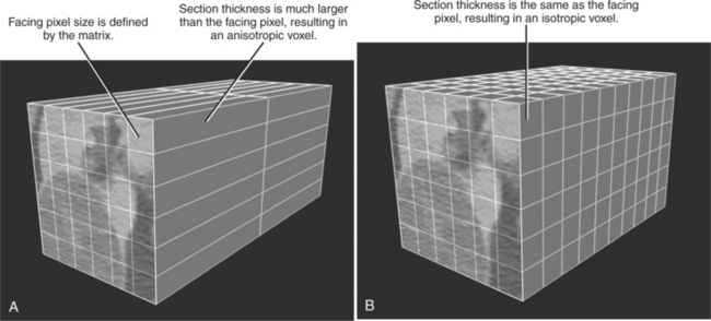
If the depth of each data component used to construct an image is considered, the square pixel is transformed into a 3D cuboid called a voxel. The depth or z-axis dimension of the voxel is defined by the value of the reconstructed section thickness. Until recently, virtually all CT and MR acquisitions yielded reconstructed voxels that were much thicker than the pixel size, usually by several fold. With the introduction of multidetector CT scanners (MDCT), particularly with 16 or more data channels, voxels can now be achieved routinely that are cubic in shape. Voxels with similar length in all three planes are called isotropic. Voxels that are not cube shaped are anisotropic (Fig. 5-1).

Figure 5-1 A, Anisotropic and (B) isotropic voxels. Axial computed tomographic section of a renal cyst superimposed over voxels represents facing pixels of an axial image with the other surfaces showing the overall dimensions of each voxel. Image is not to scale.

(Modified from Dalrymple NC, Prasad SR, Freckleton MW, Chintapalli KN: Informatics in radiology (infoRAD): introduction to the language of threedimensional imaging with multidetector CT, Radiographics 25:1409-1428, 2005, by permission.)

Voxel geometry has limited significance if axial sections alone comprise the total utilization of CT data. Because the voxel length in the z-axis is determined by reconstructed section thickness, voxel geometry does determine the degree of volume averaging that occurs (affecting image noise) but has minimal other impact on axial imaging. Such geometry, however, is one of the most crucial elements to successful application of nonaxial image processing. In general, these imaging applications may be divided into three main types: multiplanar reformations (MPRs), slab projections, and volume rendering.

MULTIPLANAR REFORMATIONS

As mentioned earlier, each axial section that comprises a CT or MR examination is created by calculating attenuation or signal values for each of its component voxels. An MPR is created by using a computer to create a new nonaxial imaging plane through the voxels of a “stacked” set of reconstructed sections. With CT, the reconstructed sections are always axial, so axial sections are stacked and a nonaxial imaging plane one voxel in thickness is defined within that volume (Fig. 5-2). With MR, the original scan data can be in any acquisition-defined imaging plane.

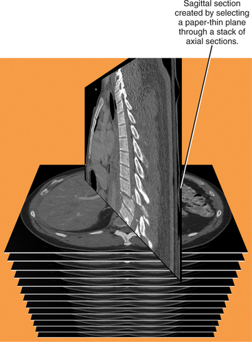
Figure 5-2 Graphic representation of how multiplanar reformations are formed.

(Modified from Dalrymple NC, Prasad SR, Freckleton MW, Chintapalli KN: Informatics in radiology (infoRAD): introduction to the language of three-dimensional imaging with multidetector CT, Radiographics 25:1409-1428, 2005, by permission.)

Choosing an Imaging Plane for Multiplanar Reformation

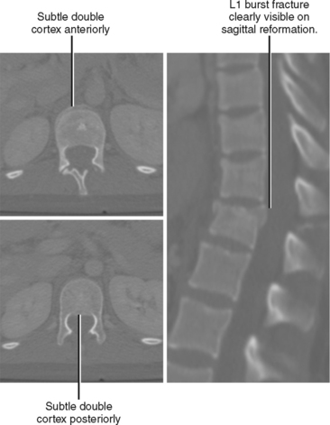
The additional perspective available with MPRs may be beneficial in two distinct ways: (1) improved lesion detection, and (2) lesion characterization. Lesion detection is improved when the structure does not lend itself to thorough evaluation in the axial plane. For example, because compressive deformity of vertebral bodies may be difficult to detect on axial sections, sagittal reformations can improve detection of spine fractures on routine abdominal CT scans (Fig. 5-3). Coronal and sagittal MPRs are helpful for the diaphragm and the hips. In most cases, the imaging plane is flat, similar to a pane of glass inserted into the volume of data.

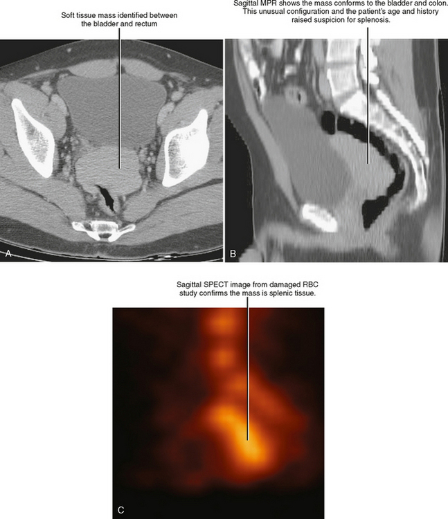
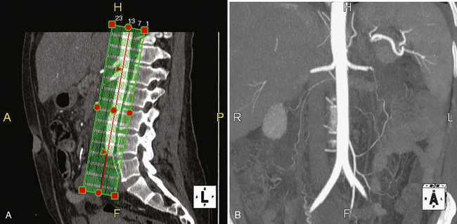
Figure 5-3 Axial and sagittal computed tomographic (CT) images of a patient with an L1 burst fracture. The fracture is visible on the axial images but could be mistaken for degenerative change. Cortical disruption and loss of vertebral body height are much more conspicuous on the sagittal reformation.

MPRs may facilitate lesion characterization by helping to identify the origin of a lesion or its shape. In some cases, MPRs are useful to characterize a specific lesion such as a suprarenal mass of uncertain origin. In other cases, the change in perspective may provide insight into the shape of a lesion, either providing a diagnosis or directing more specific investigation (Fig. 5-4). MPRs are also useful in lesion detection, such as locating an appendix not readily apparent on axial sections. Because the potential benefit of MPRs rests on an improved alignment between the orientation of the organ in question and the selected imaging plane, arbitrary imaging planes may not be the optimal choice. Oblique planes are those that are off-axis from standard axial, coronal, and sagittal planes. One of the most commonly prescribed oblique planes is a coronal oblique view of the abdominal aorta (Fig. 5-5). In certain cases, it is helpful to manipulate the imaging plane in real time to clarify issues raised during the interpretive session.

Figure 5-4 Thirty-three-year-old man with abdominal pain. Images of the upper abdomen showed a history of left nephrectomy and splenectomy for prior trauma. Pelvic malignancy was suspected on the axial images (A) initially, but sagittal reformations (B) prompted a technetium 99m (Tc-99m)–labeled heat-damaged red blood cell (RBC) study (C) that led to the correct diagnosis of trauma-related splenosis. MPR, Multiplanar reformation; SPECT, single-photon emission computed tomography.

Figure 5-5 Prescribing coronal oblique images of the abdominal aorta. A, A sagittal image through the abdominal aorta is used to select the optimal oblique plane for the aorta. B, The coronal oblique maximum intensity projection image includes the entire abdominal aorta and its major branches.

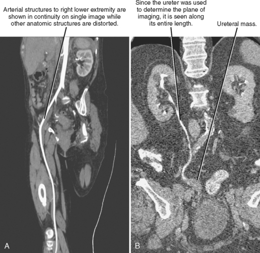
For focused evaluation of a curvilinear structure such as a blood vessel, an imaging plane may be defined that follows that one particular structure. This is a curved planar reformation (CPR), and the resulting image transforms a curved length of vessel, ureter, or intestine into a straight segment (Fig. 5-6). Because all other structures in the image are distorted by the curved imaging plane, CPR is useful only to investigate the structure used to define its imaging plane. Similar to MPRs, CPRs are a single voxel in depth.

Figure 5-6 Two examples of curved planar reformations (CPRs). A, CPR of the abdominal aorta and contiguous arterial system to level of popliteal artery. B, CPR of the right ureter in a patient with urothelial carcinoma of the ureter.

PROJECTION TECHNIQUES

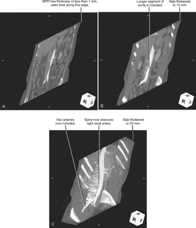
Although MPRs can provide perspective tailored to the anatomic structure or clinical question at hand, thickening the MPR into a slab of data that is two or more voxels in thickness opens the door to additional possibilities that further enhance the diagnostic value of the data (Fig. 5-7). The imaging algorithms become more complex using slabs, because utilizing the “depth” of a slab requires extrapolating a line of sight from the viewer’s eye through the slab, intersecting all voxels within the slab along that specific path. If the image is rotated, the line of sight intersects different combinations of voxels as the incident angle changes. Because the line of projection determines the appearance of the resulting image, these are called projection techniques.

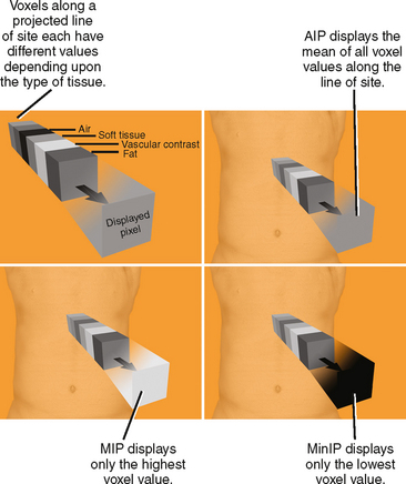
Figure 5-7 A-C, Thickening a coronal multiplanar reformation (MPR) into a slab allows application of projection techniques (maximum intensity projection in this example). This image was rotated off-axis to allow visualization of the edge of the slab.

The main benefit of thickening an MPR into a slab projection is that it incorporates multiple voxels along the line of sight to determine the displayed value. This allows the user to select from among different mathematical algorithms to determine how the collection of voxel values will be processed (Fig. 5-8). Each of these types of projection processing techniques is discussed briefly in the following sections.

Figure 5-8 Graphic representation of projection techniques. AIP, Average intensity projection; MinIP, minimum intensity projection; MIP, maximum intensity projection.

Maximum Intensity Projection

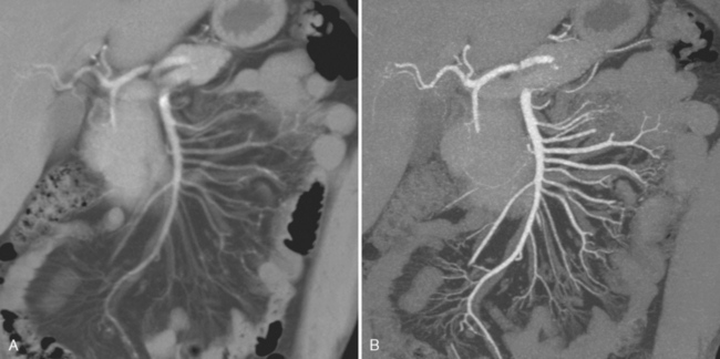
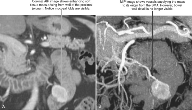
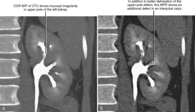
Maximum intensity projection (MIP) is perhaps the most well-known type of projection technique and one of the most commonly used. When MIP is used, of all the voxels intersected by a particular line of sight, only the one with the greatest value is represented in the image. This technique is effective at demonstrating continuous segments of high-attenuation or high-signal structures such as arteries opacified with intravascular contrast media or ureters filled with excreted contrast media (Fig. 5-9). Note that because high-intensity voxels are emphasized and low-attenuation voxels are ignored or deemphasized, evaluation of soft-tissue structures may be limited (Fig. 5-10), and small filling defects within a high-intensity lumen may be obscured (Fig. 5-11).

Figure 5-9 Effect of maximum intensity projection (MIP) technique on visualizing vascular structures opacified with contrast. A, Fifteenmillimeter slab image using ray sum. B, Same 15-mm slab using MIP displays greater detail of superior mesenteric artery and its branches.

Figure 5-10 Coronal computed tomographic images of jejunal mass surgically proven to be gastrointestinal stromal tumor. A, Average intensity projection and (B) maximum intensity projection (MIP). AIP, Average intensity projection; SMA, superior mesenteric artery.

Figure 5-11 “Blooming” of maximum intensity projection (MIP) image obscures filling defects. Coronal (COR) MIP (A) and multiplanar reformation (MPR) (B) images from excretory phase of computed tomographic urogram (CTU).

MIP first gained popularity using data from magnetic resonance angiography (MRA) but has become increasingly popular for CT applications as well. The number of images required to visualize the full length of a structure depends on the orientation and thickness of the slab, as well as how straight or tortuous the structure in question is. As with all projection techniques, the thickness and orientation of the slab are selected by the operator, and thus are likely to be of greater utility with a knowledgeable user.

Average Intensity Projection and Ray Sum

Average intensity projection (AIP) applies a different algorithm than the slab technique used by MIP. When AIP is applied to a slab, the average value of the voxels intersected by the ray of projection is used to construct the image (see Fig. 5-8). The result is an image quality similar in appearance to traditional axial sections used for CT interpretation. Similar to the way that increasing section thickness is an effective method for decreasing image noise, AIP uses thickening of the slab to decrease the noise that is otherwise present in many MPR images. A relatively thin AIP is less likely than MIP to obscure small filling defects within a segment of artery or ureter. However, a shorter segment of each artery or ureter is included in each image (see Figs. 5-9 and 5-10), decreasing the sense of continuity on the image.

Ray sum uses a different algorithm to achieve an appearance similar to AIP. As the name implies, when ray sum is applied, the sum of values within each voxel along a given ray of projection is used to construct the image. Although the mean is not obtained as in AIP, each voxel in the row defined by the line of sight influences the ultimate value; therefore, the overall result is similar and in most cases indistinguishable from AIP.

Minimum Intensity Projection

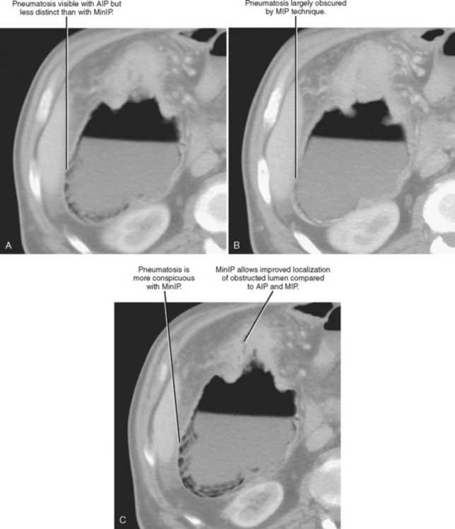
Minimum intensity projection (MinIP) is, in effect, the opposite of MIP. When MinIP is applied, of the voxels intersected by the ray of projection through a slab, only the lowest value along each ray is used to contrast the image (see Fig. 5-8). This technique emphasizes lowattenuation structures and is used most commonly for air-filled structures such as airways or regions of air trapping within the lung, although it is occasionally useful to evaluate fat or fluid within a high-attenuation object. The utility of MinIP can be illustrated by comparing the effects of MinIP with MIP and AIP techniques on the appearance of a segment of bowel with pneumatosis (Fig. 5-12). Because abnormal air can usually be detected on axial source images, MinIP is not usually necessary. However, it can be applied to increase sensitivity for small amounts of air when suspected or to further characterize indeterminate low-attenuation foci.