A Novel Combined Imaging/Morphometrical Method for the Analysis of Human Sural Nerve Biopsies for Clinical Diagnosis

Fig. 1.

(a) The nerve biopsy is placed on dental wax and kept moist with saline while portions are cut with a razor blade. (b) One of the 1.5 cm portions will be preserved in 3.6% glutaraldehyde in Millonig’s phosphate buffer, then further divided for analyses.

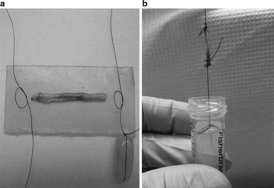
Fig. 2.

(a) One portion of the nerve is tied on each end by suture silk, (b) weighted by a glass bead and immersed into a 15 mL centrifuge tube containing fixative. The cap secures the top suture, keeping the weight from touching the bottom of the tube. This portion will be further divided, after fixation, into 1 mm³ cross-sections for morphometric and electron microscopic analysis. The remainder is reserved for teased fiber analysis.

3.2 Tissue Processing

Tissue processing chemically stabilizes the cellular constituents through fixation to preserve the morphology. The sample is then dehydrated and infiltrated with plastic resin to enable thin sectioning.

The tissue is fixed as described above and then washed in Millonig’s phosphate buffer three times for 5 min each. All solution changes should be disposed of through hazardous waste.

Postfix the nerve biopsy in 2% osmium tetroxide in Millonig’s buffer for 2 h at room temperature on a rotator in a fume hood.

Wash in Millonig’s buffer three times for 5 min each.

The following schedule is used to infiltrate and embed a specimen using a 1,000 W laboratory grade microwave oven, such as a BP-110 (Microwave Research Applications, Laurel, MD) or equivalent (7). Use approximately 4 mL of solution for each step and microwave the sample, solution, and tube in 200 mL of cold tap water for each solution change (see Notes 9 and 10).

Solution	Microwave time	Power control
Ethanol, 35%	1 min 35s	Medium low
Ethanol, 50%	1 min 35s	Medium low
Ethanol, 70%	1 min 35s	Medium low
Ethanol, 85%	1 min 35s	Medium low
Ethanol, 95%	1 min 35s	Medium low
Ethanol, 100% (5×)	1 min 35s	Medium low
Propylene Oxide (4×)	1 min 35s	Low
Propylene Oxide/Spurr’s 3:1	1 min 35s	Low
Propylene Oxide/Spurr’s 1:1	1 min 35s	Medium low
Propylene Oxide/Spurr’s 1:3	1 min 35s	Medium low
Spurr’s (100%)	1 min 35s	Medium low

Place the tissue into capsules with fresh resin and polymerize in a 70°C oven overnight.

3.3 Glass Knife Preparation

Glass knives are routinely used in ultramicrotomy and should be made according to the manufacturer’s instrument recommendations. We use 45 degree angle knives, broken from glass strips 6.4 mm × 25 mm × 400 mm and attach 6.4 mm boats from Electron Microscopy Sciences (EMS, Hatfield, PA) with nail polish.

3.4 Block Sectioning

Cut semi-thin sections 0.50–0.75 μm thick with a fresh glass knife. Trim away excess Spurr’s resin from the block face with a single edge razor blade. Make sure the final sections are free of knife marks. Use a heat pen to flatten out the compression from sectioning before transferring with a loop to a pre-cleaned, coated glass slide.

Collect several sections per slide.

Bake sections for 1 h at 70°C to ensure section adherence.

3.5 Thick Section Staining

Before proceeding with imaging and morphometric analysis, the stained thick sections must be reviewed by a pathologist to assess preservation and orientation suitability.

Filter 1% aqueous P-phenylenediamine (#42 Whatman filter paper).

Stain slides for 1–3 h at room temperature. The stain and contaminated dry waste should be disposed of as hazardous waste.

Rinse gently with running tap water for 10 min.

Differentiate and dehydrate one time with 95% ethanol for 10–15 min. Monitor this procedure through a light microscope since the stain will fade if left too long in this reagent.

Air dry and mount with a size 1½ coverslip and a resin based mounting medium using gauze to wick away any excess solution.

3.6 Confocal Microscopy Imaging

Images are acquired with a Zeiss 510 META confocal microscope (Carl Zeiss MicroImaging, LLC, Thornwood, NY). This confocal is equipped with an inverted microscope and four lasers, including a 25 mW 405 blue diode laser, a 30 mW argon gas laser with four selectable laser lines including 458, 477, 488, and 514, a 1 mW 543 helium neon gas laser, and a 5 mW 633 helium neon gas laser. The tiling will employ the 1 mW 543 helium neon gas laser. After first optimizing the image acquisition in channel mode, a low magnification automated image tiling is activated which subdivides a region of interest in a grid array without image stitching within the array. This tiling array will provide a complete overview of the sural nerve cross-section. For the final array (although a tiling array can be used at any magnification), we have selected a ×100 Plan Apochromat objective lens with a 1.4 numerical aperture. We have found the ×100 tiling provides more tiles within a fascicle with finer detail. The final tile array image will be displayed as one single image in an 8 bit (0–256) gray level scale. The display of this tile array will be shown reduced, for example, to 25% or lower to accommodate monitor display, but can be zoomed in to the original 100% pixel resolution for data analysis.

Turn on the confocal microscope system, which will include a mercury lamp, laser assembly, CPU, monitor, microscope, and electronics box.

Open the LSM510 software; “Scan new images” and “Expert mode” should be selected.

In the “Acquire” menu, select the laser dialog box and turn on the 543 laser.

Open the “Microscope” and “Stage” dialog boxes. In the “Microscope” dialog box, select the ×10 objective. For an inverted microscope, the objective will rotate into place and be raised into the work mode. Make sure both the slide and the objective are clean. If necessary, remove the objective and inspect it under a dissecting microscope to ensure it is free of debris. In the “Stage” dialog box, drop the objective down by selecting the “load” icon so that a slide can be safely placed on the stage without scratching the lens. Whenever a slide is placed on, or removed from the stage, the objective must be in the “load” mode.

Mount the slide onto the stage with the coverslip facing the objective. Select the “work” icon to move the objective up to the focus plane. In the “Microscope” dialog box, choose “Transmitted Light” “ON” (intensity 1–2) and no filters. Select the “VIS” icon from the main “Acquire” toolbar. Find a section on the slide that is well attached, unwrinkled, and stained well, without crystal artifact. Capture a single, low magnification ×10 image which will be used to measure the areas of whole fascicles and for determining the sampling scheme. Save the image.

Assign a number to each of the fascicles, for example, in a clockwise direction around the section. This can be done on a print-out of the image, or with the overlay tool in the LSM software. If using the overlay tool for numbering, the image must be saved by selecting “Export,” as image type “Contents of image window,” “single plane,” and as file type “tif” to retain the overlay information (see Fig. 3a).

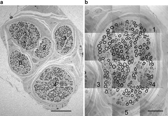
Fig. 3.

(a) Image of whole nerve cross-section, with fascicles numbered. (b) Whole tiled image of first fascicle (fascicle #3) chosen by random number start. Each tile retains its 100% pixel resolution (1,024 × 1,024) captured with a ×100 oil immersion objective lens. Numbers indicate systematic uniform random sampling (SURS) results. Scale bar = 200 μm (a); 50 μm (b).

Go to www.random.org and generate a random number (RN) between 1 and the total number of fascicles. The result will be the first fascicle to tile. Renumber the remaining fascicles, choose another random number between 1 and the remaining number of fascicles. The result is the second fascicle to tile. Continue with this system until all fascicles have been chosen and ordered for imaging.

Center the first fascicle to image in the field of view. Select the “load” mode and remove the slide.

Rotate the ×100 objective into place and again drop the objective into load mode. If your objective is a DIC objective, the DIC slider can be removed from the objective since the intent is to capture a simple grayscale image.

10.

Put a drop of fluorescence free immersion oil (Zeiss Immersol 518F, Carl Zeiss MicroImaging) on the coverslip and secure the slide with clips to hold the slide when tiling. In the “Stage” dialog box, select the “work” icon to move the objective up to the focus plane. Bring the image sharply into focus and perform Koehler illumination (see Note 11).

11.

From the “Acquire” menu open the “Configure” and “Scan” dialog boxes. In “Configure,” select “Channel Mode” and “Single Track.” Select “Channel D” at the bottom of the dialog box and uncheck any other detectors selected. In the “Scan” window, select “Mode,” then frame size 1,024 × 1,024 with no line/frame averaging, 8 bit (in a tile scan, the program defaults to this even if 12 bit is selected), single scan direction, a zoom factor of 1, and a scan speed of 5 or 6. Then select the “Channels” page from the “Scan” window and activate the 543 laser excitation wavelength at 80%. Click the “XY Continuous” button, fine focus for the laser, and adjust the channel settings for gain and offset using the range indicator to more accurately monitor the intensity changes. The range indicator is found on the image toolbar in the artist palate icon. It will pseudocolor any pixels with an intensity value near 0 (black) as blue and any pixels with an intensity value near 255 (white) as red. All other pixel values are displayed in grayscale. Care should be taken when adjusting the detector gain and offset to avoid pixel intensities in the red or blue range.

12.

Once the gain and offset parameters are optimally set, in the “Scan” dialog box select “Mode,” then frame size 128 × 128 with no line/frame averaging, 8 bit, single scan direction, and a zoom factor of 1 and the fastest scan speed allowed. In the “Stage” dialog box, set the estimated number of tiles to cover the fascicle, the stage speed to 1, then Start. View the results and click on the “move to” box in the stage control dialog box and move the white box on the tiled image to the estimated center of the section. Adjust the tile numbers either in the x or y dimension to include the entire nerve fascicle. Repeat if necessary until the fascicle is completely represented and centered.

13.

For a final tile scan, reset the frame size to 1,024 × 1,024 and scan speed to 6 or 7. Click Start from the “Stage” dialog box. When the tiling is finished, save the image with sample identification and fascicle order in the file name (first, second, etc.) (see Note 12) (see Fig. 3b). Capture a tiled image for every fascicle, again including its order in the file name.

3.7 MetaMorph Image Analysis

Analysis is performed using MetaMorph offline software version 7.7.3 64 bit (Molecular Devices, Sunnyvale, CA). Interpretation of the morphometric analyses of sural nerve biopsies will be performed by the requesting pathologist. MetaMorph software will read the calibration information directly from the LSM image as the calibration is calculated from the objective magnification, pixel size, and zoom factor included in the “meta data” file header.

Open the MetaMorph software and go to Edit-Preferences. In “Preferences,” select the “Measure Objects” tab and select “Measure all regions” and “Log summary data on single line.”

Select “Measure” menu, and “Region Measurements” to configure measurement and logging choices:

Include: All regions
Configure Tab: Select “Disable All” then check “Region Label,” “Image Name,” and “Area”
Display and Log: check “Region Measurements Only”
Check “Log Image Calibration”
Check “Log Column Titles”
Select “Open Log”: Log measurements to: Dynamic Data Exchange (DDE)-OK

Export Log Data Dialog Box
Application: Microsoft Excel
Sheet name: Sheet1
Starting Row: 1
Starting Column: 1
OK (see Note 13)

Open the low magnification LSM image of the entire nerve biopsy cross-section. The calibration should load automatically. Always check the bottom of the screen to be sure the correct calibration file has been loaded. Using the “Trace Region” tool, measure each fascicle area. Log to spreadsheet. View the logging results, save the spreadsheet, and minimize this screen area.

Open a tiled LSM image of the first fascicle to analyze. Using the random number generator, locate and center the first tile to be analyzed. Select the “Rectangular Region” tool and create a rectangular region defining this tile (8,100 μm² for a 1,024 × 1,024 tile using a ×100 lens), or go to the region tool properties and under region size, type in pixel dimensions to match the image acquisition resolution (e.g., 1,024 × 1,024). Then, with the “Rectangular Region” tool activated, click on the upper left corner of the tile and it will be outlined automatically. Set zoom to 33%.

With rectangular region activated (pulsing border), go to the “Display” menu-“Graphics”-“Grid.” Set values in “Draw Grid” dialog box to draw 3 × 3 boxes on “Selected Image,” with a line thickness of 3, Color 255. Click “Draw Grid.” Delete active region.

A grid with nine boxes will be overlaid on this ROI. Measurements will be made in the center box, which will function as the unbiased counting frame, while the surrounding eight boxes will be used as the guard area (see Note 14) (see Fig. 4 and 5). The term “counting frame” is referencing only the center box of the grid overlay.

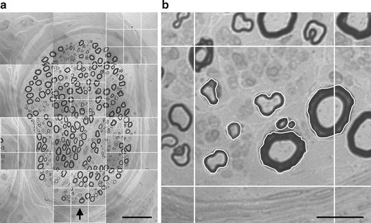
Fig. 4.

(a) First fascicle with grid overlays. The center box of each 9 × 9 grid overlay functions as the unbiased counting frame for each tile within which to measure endoneurial/reference area (RA) and the area of each allowed MFP. (b) Center box of the grid overlay, as the unbiased counting frame from the fifth ROI/tile, with allowed MFPs traced. Scale bar = 50 μm (a); 10 μm (b).

Only gold members can continue reading. Log In or Register to continue