a Path for Segmentation Through Sequential Learning

and $p(S|I) = \prod _x p(S(x)|I(\mathcal {N}(x)))$ , where $\mathcal {N}(x)$ is a neighborhood surrounding x and $I(\mathcal {N}(x))$ is the image features extracted from the neighborhood. Given the estimated probabilities, the maximum a posterior (MAP) segmentation can be derived as $S(x)=\mathrm {argmax}_l p(l|I(\mathcal {N}(x)))$ .

2.2 Complexity of Image Segmentation

Under the probabilistic view, each segmentation problem can be modeled by classifiers learned from training data. Hence, the complexity of a segmentation problem can be measured by the complexity of the corresponding classification problem. We define the complexity of a segmentation problem as follows:

$\begin{aligned} H(D) = H(D;C) + H(D|C) \end{aligned}$

(1)

where

are data extracted from training images with $F=\{f_1,...,f_n\}$ specifying feature representations of n samples and $Y=\{y_1,...,y_n\}$ specifying the segmentation labels. C is a classifier. H(D; C) is the information about the segmentation problem captured by C. H(D|C) is the residual information not captured by classifier C, which can be defined as:

$\begin{aligned} H(D|C) = \frac{1}{n}\sum _{i=1}^n - \log p(y_i|f_i,C) \end{aligned}$

(2)

where

is the label posterior computed by C using feature

In the literature, classifier complexity H(C) is often described as the complexity of decision boundaries. Many factors may affect classifier complexity. The most influential factors include features and the learning model, e.g. linear or nonlinear. When a classifier accurately models a classification problem,

. Due to overfitting, it is common that

and

$$H(D|C)>0$$” src=”/wp-content/uploads/2016/09/A339424_1_En_38_Chapter_IEq13.gif”></SPAN>. When overfitting is minimized, e.g. through techniques such as cross-validation, the complexities of two segmentation problems can be approximately compared by the residual terms, given that the modeling classifiers for the two problems have similar complexities, e.g. both trained by the same learning model using same image features. If <SPAN class=EmphasisTypeItalic>p</SPAN>(<SPAN class=EmphasisTypeItalic>l</SPAN>|<SPAN class=EmphasisTypeItalic>f</SPAN>, <SPAN class=EmphasisTypeItalic>C</SPAN>) is narrowly peaked around its maximum for each data, there is little residual information. In contrast, if the distribution is flat or multiple modes are widely scattered, the segmentation problem is more complex as more residual information is not captured by <SPAN class=EmphasisTypeItalic>C</SPAN>.</DIV></DIV><br />
<DIV id=Sec5 class=

2.3 Bayesian Approximation

Under the Bayesian rule, the posterior label probability distribution of a target segmentation can be computed as:

$\begin{aligned} p(l|I,x)=\int _{S'}p(S'|I,C^1)p(l|I,S',x) \end{aligned}$

(3)

index through all possible segmentations for I. $$p(S'|I,C^1)$$

is the probability of a segmentation given the observed image I as modeled by classifier $$C^1$$

Although it is intractable to enumerate all feasible segmentations in (3), accurate approximation exists when certain conditions are satisfied. When $$p(S'|I,C^1)$$

is narrowly peaked around its maximum, a commonly applied approximation is based on the MAP segmentation, e.g. [11]:

$\begin{aligned} p(l|I,x)\sim p(S^1|I,C^1)p(l|I,S^1,x)\propto p(l|I,S^1,x) \end{aligned}$

(4)

where

is the MAP segmentation derived from $$C^1$$

. The condition also means that the underlying segmentation problem modeled by $$C^1$$

can be reliably solved by $$C^1$$

. If the condition is not satisfied, the MAP solution has larger variations, which results in greater mismatch between features extracted from $$S^1$$

during training and testing. This limitation makes learning more easily prone to overfitting, reducing the benefit of adding $$S^1$$

as additional features. Since $$p(S^1|I,C^1)$$

is a constant scale factor, to solve the original segmentation problem, we only need to estimate $$p(l|I,S^1,x)$$

. As shown in [6, 9, 13], when $$S^1$$

is correlated with the target segmentation, it provides contextual information, such as shape or spatial relations between neighboring anatomical regions, that is not captured by local image features.

The above approximation has an intuitive interpretation. A segmentation problem may be solved through transferring it into a simpler segmentation problem that can be solved with less ambiguity. Solving the simplified segmentation problem first may help solving the original segmentation problem.

A Case Study: Corrective learning [13] applies classification techniques to correct systematic errors produced by a host segmentation method with respect to some gold standard segmentation. In our context, the segmentation produced by the host method is a MAP solution. In corrective learning, the classifiers trained for making corrections aim to estimate label posteriors given the observation of the image and the segmentation produced by the host method, i.e. $$p(l|I,S^1,x)$$

. Hence, corrective learning is in fact an application of the MAP approximation (4). The fact that corrective learning achieves better performance than learning purely based on image features on some previous studies indicates the effectiveness of the MAP-based approximation. Our study suggests that corrective learning may work even more effectively when the host method aims to solve a simplified segmentation problem derived from the target segmentation problem.

2.4 Iterative Extension: Finding a Path to Segmentation

The approximation in (4) can be recursively expanded. Hence, we have:

$\begin{aligned} p(l|I,x)\sim & {} p(S^1|I,C^1)p(l|I,S^1,x) \end{aligned}$

(5)

$\begin{aligned}\sim & {} p(S^1|I,C^1)p(S^2|I,S^1,C^2)p(l|I,S^1,S^2,x) \end{aligned}$

(6)

$\begin{aligned}\sim & {} p(S^1|I,C^1)\dots p^n(S^n|I,S^1,...,S^{n-1},C^{n})p(l|I,S^1,...,S^n,x)\end{aligned}$

(7)

$\begin{aligned}\propto & {} p(l|I,S^1,...,S^n,x) \end{aligned}$

(8)

are trained classifiers and $$S^i$$

is the MAP solution derived from $$C^i$$

For this approximation to be accurate, a necessary condition is that for each $1< i\le n$ , $$S^i$$

can be computed with little ambiguity with $C^{i}$ given the image I and the MAP segmentations obtained from previous iterations, i.e. $\{S^1,\dots ,S^{i-1}\}$ . To allow solving the original segmentation problem benefit from this approximation, an additional requirement is that each $$S^i$$

must provide additional information about the desired segmentation that is not already captured by I and $\{S^1,\dots ,S^{i-1}\}$ . In other words, $$S^i$$

should be more similar to the desired segmentation as i increases. Under these requirements, $$(C^1$$

,…,

defines a path for solving the original segmentation problem. Each $$C^i$$

aims to accurately solve a simplified segmentation problem. As i increases, the complexity of the problem solved by $$C^i$$

also increases.

2.5 The Path Learning Algorithm

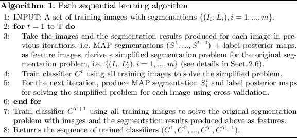
To implement the sequential learning model in (7), we propose an iterative extension to the corrective learning method [13]. The motivation for building the implementation based on corrective learning is that corrective learning is designed to be more effective in utilizing segmentation results produced in previous iterations for building stronger segmentation classifiers.

For step 4 at each iteration t, we train AdaBoost classifiers [4] to solve the simplified segmentation. First, we define a working region of interest (ROI) for each label by performing dilation to the set of all voxels assigned the label in the MAP segmentation produced in the previous iteration, i.e. $S^{t-1}$ . Using instances uniformly sampled within a label’s working ROI, one AdaBoost classifier is trained to identify voxels assigned to this label against voxels assigned to other labels in the target segmentation within the ROI. To apply these classifiers on a testing image, each classifier is applied to evaluate the confidence of assigning the corresponding label to each voxel within the label’s working ROI. If a voxel belongs to the ROI of multiple labels, the label whose classifier gives the maximal posterior at the voxel is chosen for the voxel. At the first iteration, if no segmentation has been produced yet, the AdaBoost classifiers are trained without using working ROIs.

Three types of features are applied to describe each voxel, including spatial, appearance, and contextual features. The spatial features are computed as the relative coordinate of each voxel to the ROI’s center of mass. The appearance features are derived from the voxel’s neighborhood patch from the training image(s). The contextual features are extracted from the voxel’s neighborhood patch from all MAP segmentations and spatial label probability maps produced in previous iterations. To enhance spatial correlation, the joint spatial-appearance and joint spatial-contextual features are also included by multiplying each spatial feature with each appearance and contextual feature, respectively. If no segmentation has been produced yet, only the appearance features will be applied.

Stacking Learning: Another issue we need to address is that sequential learning is more prone to the overfitting problem. Due to overfitting, the intermediate segmentation results produced for a testing image may be different from those produced for training images. Since these segmentation results are applied as features in subsequent iterations, this training/testing mismatch will compromise the performance of the classifiers learned in subsequent iterations. To alleviate this problem, we apply the stacking technique [3, 7, 15] (at step 5 in the above algorithm). For training, the MAP segmentation produced for each training image is produced from cross-validation.

Only gold members can continue reading. Log In or Register to continue