Adaptive Color Image Processing

ab representation have been introduced to overcome these limitations [8].

In this chapter, both the RGB, L

and HSL (hue/saturation/luminance) color space representations will be used for defining spatially adaptive color image filters. The CIE L

color space is deduced from the CIE XYZ color space:

$\begin{aligned} \left\{ \begin{array}{lll} L^*&{}=&{}116f(Y/Y_n)-16,\\ a^*&{}=&{}500(f(X/X_n)-f(Y/Y_n)),\\ b^*&{}=&{}200(f(Y/Y_n)-f(Z/Z_n). \end{array}\right. \end{aligned}$

(1)

where:

$$$\begin{aligned} f(t)=\left\{ \begin{array}{ll} \displaystyle t^{\frac{1}{3}}&{}\mathrm{if }\,\, \displaystyle t >\left( \frac{6}{29}\right) ^3,\\ \displaystyle \frac{1}{3}\left( \frac{29}{6}\right) ^2 t+\frac{4}{29}&{}\mathrm{ otherwise }. \end{array}\right. \end{aligned}$$” src=”/wp-content/uploads/2016/03/A308467_1_En_6_Chapter_Equ2.gif”></DIV></DIV><br /> <DIV class=EquationNumber>(2)</DIV></DIV>Here <SPAN id=IEq10 class=InlineEquation><IMG alt=$ and $$Z_n$$

are the CIE XYZ tristimulus values of the reference white point corresponding to the illuminant $$D65$$

The HSL space is derived from the RGB space by the following equations:

$$$\begin{aligned} \left\{ \begin{array}{lll} \displaystyle H&{}=60^{\circ }\times &{}\left\{ \begin{array}{lll} \displaystyle \frac{G-B}{\max (R,G,B)-\min (R,G,B)}&{}\mathrm{ if }&{}R=\max (R,G,B),\\ \displaystyle \frac{B-R}{\max (R,G,B)-\min (R,G,B)}+2&{}\mathrm{ if }&{}G=\max (R,G,B),\\ \displaystyle \frac{R-G}{\max (R,G,B)-\min (R,G,B)}+4&{}\mathrm{ if }&{}B=\max (R,G,B). \end{array}\right. \\ S&{}=&{}\left\{ \begin{array}{lll} \displaystyle \frac{\max (R,G,B)-\min (R,G,B)}{\max (R,G,B)+\min (R,G,B)}&{}\mathrm{ if }&{}L\le 0.5,\\ \displaystyle \frac{\max (R,G,B)-\min (R,G,B)}{2-\max (R,G,B)-\min (R,G,B)}&{}\mathrm{ if }&{}L>0.5. \end{array}\right. \\ \displaystyle L&{}=&{}\displaystyle \frac{\max (R,G,B)+\min (R,G,B)}{2} \end{array}\right. \end{aligned}$$” src=”/wp-content/uploads/2016/03/A308467_1_En_6_Chapter_Equ3.gif”></DIV></DIV><br /> <DIV class=EquationNumber>(3)</DIV></DIV></DIV><br /> <DIV></DIV><br /> <DIV id=Sec4 class=$

1.3 Need of Vector Order Relations

Rank-order filters (such as morphological filters or Choquet filters) need the use of an order relation between the intensities to be processed. The application of rank-order filtering to color images is not straightforward due to the vectorial nature of the color data. Several vector order relations have been proposed in the literature such as marginal ordering, lexicographical ordering, partial ordering and reduced ordering [2, 6]. For example, let $E=A\times B\times C$ be a color space where $$A, B, C$$

are three sets of scalar values. The lexicographical order on $$E$$

, denoted $\prec _E$ , with the component ordering $A\rightarrow B\rightarrow C$ is defined as following for two color vectors $$c_1=(c_1^A,c_1^B,c_1^C)$$

and

$\begin{aligned} c_1\prec _E c_2 \Leftrightarrow \left\{ \begin{array}{l} c_1^A<c_2^A {\text { or}},\\ c_1^A=c_2^A {\text { and }} c_1^B<c_2^B {\text { or}},\\ c_1^A=c_2^A {\text { and }} c_1^B=c_2^B {\text { and }}\, c_1^C<c_2^C. \end{array} \right. \end{aligned}$

(4)

Concerning the vectorial ordering, the lexicographical one will be used in this chapter by fixing the ordering of the components for the three color space representations as follows:

in RGB: $R\rightarrow G \rightarrow B$ or $G\rightarrow R \rightarrow B$
in Lab: $L^*\rightarrow a^* \rightarrow b^*$
in HSL: $(H\div h_0) \rightarrow S \rightarrow L$ or $L\rightarrow S \rightarrow (H\div h_0)$ where corresponds to the origin of hues and $\div$ denotes the angular difference defined as:
$$$\begin{aligned} h_1\div h_2=\left\{ \begin{array}{lll} |h_1-h_2|&{} \mathrm{ if } &{}|h_1-h_2|\le 180^{\circ },\\ 360^{\circ }-|h_1-h_2|&{} \mathrm{ if } &{}|h_1-h_2|> 180^{\circ }.\\ \end{array}\right. \end{aligned}$$” src=”/wp-content/uploads/2016/03/A308467_1_En_6_Chapter_Equ5.gif”></DIV></DIV><br /> <DIV class=EquationNumber>(5)</DIV></DIV></DIV></LI></UL></DIV>In the literature, several approaches combining color representations and order relations have been proposed for defining nonlinear color image filters [<CITE><A href=$ 2, 4, 5, 19, 27, 32, 37–39].

2 Color Adaptive Neighborhoods (CANs)

This chapter deals with 2D color images, that is to say image mappings defined on a spatial support in the Euclidean space $\mathbb {R}^2$ and valued onto a color space $E\subseteq \mathbb {R}^3$ (such as RGB, Lab, HSL…). The set of color images is denoted ${\mathop {{\fancyscript{I}}}}$ .

2.1 Definition

In order to process color images within the GANIP framework, it is first necessary to define Color Adaptive Neighborhoods (CANs) in the most simple way.

For each point $x\in D$ and for a color image $f_0\in {\mathop {{\fancyscript{I}}}}$ , called the pilot image, the CANs denoted $V_{m}^{f_0}(x)$ are subsets in . They are built upon in relation with a homogeneity tolerance belonging to the positive real value range $\mathbb {R}^+$ . More precisely, $V_{m}^{f_0}(x)$ is a subset of which fulfills two conditions:

1.

its points have a color value close to that of the point : $\forall y \in V_{m}^{f_0}(x)\quad {||f_0(y)- f_0(x)||}_E\le m$ , where denotes a functional on the color space . By using the RGB, Lab and HSL color spaces, the functionals are defined as [2]:

$\begin{aligned} {||c_1-c_2||}_{RGB}&=\sqrt{{(c_1^R-c_2^R)}^2+{(c_1^G-c_2^G)}^2+{(c_1^B-c_2^B)}^2}\end{aligned}$

(6)

$\begin{aligned} {||c_1-c_2||}_{L^*a^*b^*}&=\sqrt{{(c_1^{L^*}-c_2^{L^*})}^2+{(c_1^{a^*}-c_2^{a^*})}^2+{(c_1^{b^*}-c_2^{b^*})}^2}\end{aligned}$

(7)

$\begin{aligned} {||c_1-c_2||}_{HSL}&=\sqrt{{(c_1^L-c_2^L)}^2 + {(c_1^S)}^2+{(c_2^S)}^2-2c_1^S c_2^S \cos (c_1^H\div c_2^H)} \end{aligned}$

(8)

2.

the set is path-connected with the usual Euclidean topology on $D\subseteq \mathbb {R}^2$ (a set is connected if for all $x_1,x_2\in X$ there exists a continuous mapping $\tau :[0,1]\rightarrow X$ such that $\tau (0)=x_1$ and $\tau (1)=x_2$ ).

The CANs are thus mathematically defined as following:

$\forall (m,f_0,x) \in \mathbb {R}^+\times {\mathop {{\fancyscript{I}}}}\times D$

$\begin{aligned} V_{m}^{f_0}(x) = C_{\{y\in D;{||f_0(y)- f_0(x)||}_E\le m\}}(x) \end{aligned}$

(9)
where denotes the path-connected component (with the usual Euclidean topology on $D\subseteq \mathbb {R}^2$ ) of $X\subseteq D$ containing $x\in D$ .

The definition of ensures that $x\in V_{m}^{f_0}(x)$ for all $x\in D$ .

2.2 Illustration

Figure 1 illustrates the CANs of two points computed on a human retina image (used ad the pilot image ). The figure highlights the homogeneity and the correspondence of the CANs with the spatial structures.

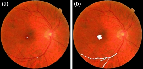
Fig. 1

a Original image with two seed points and (white dots). b CANs $V_{25}^{f_0}(x)$ and $V_{25}^{f_0}(y)$ . The CANs of the two selected points of the original color image are homogeneous with the tolerance in the RGB color space

2.3 Properties

These color adaptive neighborhoods satisfy several properties:

1.

reflexivity:

$\begin{aligned} x \in V_{m}^{f_0}(x) \end{aligned}$

(10)

2.

increasing with respect to :

$\begin{aligned} \left( \begin{array}[c]{l} (m_1,m_2) \in \mathbb {R}^+\times \mathbb {R}^+\\ m_1 \le m_2 \end{array} \right) \Rightarrow V_{m_1}^{f_0}(x) \subseteq V_{m_2}^{f_0}(x) \end{aligned}$

(11)

3.

equality between iso-valued points:

$\begin{aligned} \left( \begin{array}[c]{l} (x,y) \in D^2\\ x \in V_{m}^{f_0}(y)\\ f_0(x)=f_0(y) \end{array} \right) \Rightarrow V_{m}^{f_0}(x) = V_{m}^{f_0}(y) \end{aligned}$

(12)

The proofs of these properties are similar to those stated for gray-tone images [11].
3 CAN Choquet Filtering

Fuzzy integrals [9, 36] provide a general representation of image filters. A large class of operators can be represented by those integrals such as linear filters, morphological filters, rank filters, order statistic filters or stack filters. The main fuzzy integrals are Choquet integral [9] and Sugeno integral [36]. Fuzzy integrals integrate a real function with respect to a fuzzy measure.
3.1 Fuzzy Integrals

Let be a finite set. In discrete image processing applications, represents the pixels within a subset of the spatial support of the image (an image window). A fuzzy measure, $\mu$ , over $X=\{x_0,\dots , x_{K-1}\}$ is a function $\mu :2^X\rightarrow [0,1]$ such that:

$\mu (\emptyset )=0;\mu (X)=1$

$\mu (A)\le \mu (B) \mathrm if A\subseteq B$
Fuzzy measures are generalizations of probability measures for which the probability of the union of two disjoint events is equal to the sum of the individual probabilities.

The discrete Choquet integral of a function $f:X=\{x_0,\dots , x_{K-1}\}\rightarrow E\subseteq \mathbb {R}$ with respect to the fuzzy measure $\mu$ is [26]:

$\begin{aligned} C_{\mu }(f)=\sum _{i=0}^{K-1}\left( f(x_{(i)})-f(x_{(i-1)}) \right) \mu (A_{(i)}) =\sum _{i=0}^{K-1}\left( \mu (A_{(i)})-\mu (A_{(i+1)}) \right) f(x_{(i)}) \end{aligned}$

(13)
where the subsymbol indicates that the indices have been permuted so that: $0=f(x_{(-1)})\le f(x_{(0)})\le f(x_{(1)})\le \dots ,\le f(x_{(K-1)}), A_{(i)}=\{x_{(i)},\dots , x_{(K-1)}\}$ and $A_{(K)}=\emptyset$ .

An interesting property of the Choquet fuzzy integral is that if $\mu$ is a probability measure, the fuzzy integral is equivalent to the classical Lebesgue integral and simply computes the expectation of with respect to $\mu$ in the usual probability framework.

The fuzzy integral is a form of averaging operator in the sense that the value of a fuzzy integral is between the minimum and maximum values of the function to be integrated.
3.2 Classical Choquet Filters

Let be a color image in $\fancyscript{I}$ , a window of points and $\mu$ a fuzzy measure defined on . This measure could be extended to all translated window associated to a pixel : $\forall A\subseteq W_y\quad \mu (A)=\mu (A_{-y}), A_{-y}\subseteq W$ . In this way, the Choquet filter associated to is defined by:

$\begin{aligned} \forall y\in D \quad CF_{\mu }^W(f)(y)= \sum _{x_i\in W_y}(\mu (A_{(i)})-\mu (A_{(i+1)}) )f(x_{(i)}) \end{aligned}$

(14)
where the subsymbol indicates that the indices have been permuted so that: $0=f(x_{(-1)})\prec _E f(x_{(0)})\prec _E f(x_{(1)})\prec _E \dots ,\prec _E f(x_{(K-1)}), A_{(i)}=\{x_{(i)},\dots , x_{(K-1)}\}$ and $A_{(K)}=\emptyset$ .

Note that $(\mu (A_{(i)})-\mu (A_{(i+1)}) )f(x_{(i)})$ corresponds to the multiplication by $(\mu (A_{(i)})-\mu (A_{(i+1)}) )$ of each component of $f(x_{(i)})$ (which is an element of the color space ). The same mapping is realized for the sum $\sum$ . In this way, the resulting value $CF_{\mu }^W(f)(y)$ is guaranteed to be in .

The Choquet filters generalize [18] several classical filters:

linear filters (mean, Gaussian, …): $LF_W^{\alpha }(f)(y)=\sum \nolimits _{x_i\in W_y}\alpha _i f(x_i)$ where $\alpha \in [0,1]^K,\sum \nolimits _{i=0}^{K-1}\alpha _i=1$

rank filters (median, min, max, …): $RF_W^{d}(f)(y)=f(x_{(d)})$ where $d \in [0,K-1]\cap \mathbb {N}$

order filters (-power, $\alpha$ -trimmed mean, quasi midrange, …): $OF_W^{\alpha }(f)(y)=\sum \nolimits _{x_i\in W_y}\alpha _i f(x_{(i)})$ where $\alpha \in [0,1]^K,\sum \nolimits _{i=0}^{K-1}\alpha _i=1$
The mean, rank and order filters are Choquet filters with respect to the so-called cardinal measures: $\forall A,B\subseteq W\quad \#A=\#B\Rightarrow \mu (A)=\mu (B)$ ( $\#B$ denoting the cardinal of ). Those filters, using an operational window , could be characterized with the application: $\#A\mapsto \mu (A), A\subseteq W$ . Indeed, different cardinal measures could be defined for each class of filters:

mean filter: $\mu$ is the fuzzy measure on defined by $\mu (A)=\#A/\#W$

rank filters: (of order ): $\mu$ is the fuzzy measure on defined by: $\mu (A)=\left\{ \begin{array}{ll} 0 &{} \mathrm{if } \, \#A\le \#W-d,\\ 1 &{} \mathrm{otherwise }. \end{array}\right.$

order filters: $\mu$ is the fuzzy measure on defined by $\mu (A)=\sum \nolimits _{j=0}^{\#A-1}\alpha _{\#W-j}$
In this way, there is a natural link between the weights $\alpha _i$ of the general order filters and the fuzzy cardinal measures: $\alpha _{\#W-i+1}=\mu _{i}-\mu _{i-1}$ where $\mu _{i}$ corresponds to the fuzzy measure of the set with cardinal $\#i$ .

For example, the median filter (using a $3\times 3$ window) is characterized by the following cardinal measure (Fig. 2):

$\begin{aligned} \forall A\subseteq W \quad \mu (A)=\left\{ \begin{array}{ll} 0 &{}\mathrm{if }\,\#A\le \left\lfloor \#W/2\right\rfloor ,\\ 1 &{}\mathrm{otherwise }. \end{array}\right. \end{aligned}$
where $\left\lfloor z\right\rfloor$ denotes the largest integer not greater than (floor).

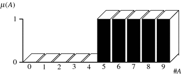
Fig. 2

Fuzzy measure of the classical median filter on a $3\times 3$ operational window [16]. The corresponding weights of this order filter are equal to $\alpha _5=\mu _5-\mu _4=1$ and otherwise

The Fig. 3 shows an illustration of several classical filters within the RGB color space, using the square of size $7\times 7$ as operational window and the lexicographical order $R\rightarrow G\rightarrow B$ . The filters are performed on a painting image of the artist Gamze Aktan.

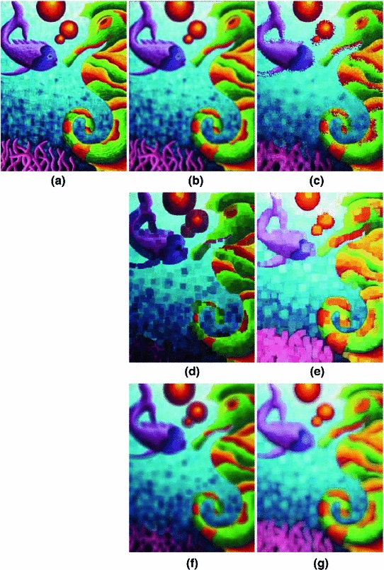
Fig. 3

a Original image. b Classical mean filtering. c Classical median filtering. d Classical min filtering. e Classical max filtering. f Classical -power filtering. g Classical $\frac{1}{3}$ -power filtering. Several classical Choquet filters within the RGB color space, using the square of size $7\times 7$

Only gold members can continue reading. Log In or Register to continue

Share this:
Click to share on Twitter (Opens in new window)
Click to share on Facebook (Opens in new window)

Related posts:

to: On the von Kries Model: Estimation, Dependence on Light and Device, and Applications Saliency Evaluation for Video Game Design Color Misalignment Correction for Close-Range and Long-Range Hyper-Resolution Multi-Line CCD Images Categorization Models for Color Image Segmentation Taxonomy of Color Constancy and Invariance Algorithm Detection and Segmentation in Color Images

Stay updated, free articles. Join our Telegram channel