Fig. 1
PET images in different views: a Coronal view; b Sagittal view; c Horizontal view; d 3D view
PET scans rely on the injected radiotracers which circulate inside the body. PET scanner detects the pairs of gamma photons emitted from the radiotracer, which are known as positron annihilation, and creates a projection data of radiotracer distribution. The reconstructed images from projection data are used for diagnosis. PET images of different views from a volunteer are shown in Fig. 1. One currently used PET radiotracer for daily clinical routines is  F-FDG (Fluoro-2-deoxy-d-glucose), which is a compound consist of glucose and radioactive fluorine-18. When disease occurs, the activities of cells begin to change, for example, the cancer cells need more glucose and more active than normal cells, so there will be more radiolabeled
  F-FDG accumulated in the cancer cells. With the PET images, it appears higher intense than surrounding tissues, which is called as a ‘hot spot’ indicating a high level of activity or metabolism is occurring there. Correspondingly, a ‘cold spot’ refers to the area of low metabolic activities indicated by lower intense in the PET images. With these PET images, doctors will be able to evaluate the working situation of organs and tissues and determine the abnormals by analyzing the hot spots and cold spots. The ability of detecting cellular level change that occurs early in the disease makes PET imaging superior to the CT and MR images which show the structural change after accumulations in cellular level. Hybrid PET/CT or PET/MRI is the combination of PET and CT or MRI, the combination of multiple imaging modalities allows both anatomical and functional images in one image set. One example of PET/CT images is shown in Fig. 2.
F-FDG (Fluoro-2-deoxy-d-glucose), which is a compound consist of glucose and radioactive fluorine-18. When disease occurs, the activities of cells begin to change, for example, the cancer cells need more glucose and more active than normal cells, so there will be more radiolabeled F-FDG accumulated in the cancer cells. With the PET images, it appears higher intense than surrounding tissues, which is called as a ‘hot spot’ indicating a high level of activity or metabolism is occurring there. Correspondingly, a ‘cold spot’ refers to the area of low metabolic activities indicated by lower intense in the PET images. With these PET images, doctors will be able to evaluate the working situation of organs and tissues and determine the abnormals by analyzing the hot spots and cold spots. The ability of detecting cellular level change that occurs early in the disease makes PET imaging superior to the CT and MR images which show the structural change after accumulations in cellular level. Hybrid PET/CT or PET/MRI is the combination of PET and CT or MRI, the combination of multiple imaging modalities allows both anatomical and functional images in one image set. One example of PET/CT images is shown in Fig. 2.Different radiotracers will reveal different diseases. Besides  F-FDG mentioned before, which is widely used for cancer diagnosis, cardiology, neurology, there are many other radiotracers used in research and clinical applications.
  F-FLT (3
 -fluoro-3
 -deoxy-l-thymidine) is developed as a PET tracer to image tumor cell proliferation [12],
  C-Acetate is developed to localize prostate cancer [62],
  N-ammonia is developed to quantify the myocardial blood flow [48],
  C-dihydrotetrabenazine (DTBZ) is developed for brain imaging, which can be used for differentiating Alzheimer’s disease from dementia and Parkinson’s disease [47],
  C-WIN35,428 is a cocaine analogue and sensitive to the dopamine transporters [93]. Researchers are working on labeling different drugs with radioactive
  F,
F,  C,
C,  N etc. for PET scan, and pharmaceutical companies are especially interested in applying quantitative PET analysis on radio-labeled new drugs, this has the potential to shorten the Phase I to Phase II studies from more than 5 years to be 2 years.
F-FDG mentioned before, which is widely used for cancer diagnosis, cardiology, neurology, there are many other radiotracers used in research and clinical applications. F-FLT (3-fluoro-3-deoxy-l-thymidine) is developed as a PET tracer to image tumor cell proliferation [12], C-Acetate is developed to localize prostate cancer [62], N-ammonia is developed to quantify the myocardial blood flow [48], C-dihydrotetrabenazine (DTBZ) is developed for brain imaging, which can be used for differentiating Alzheimer’s disease from dementia and Parkinson’s disease [47], C-WIN35,428 is a cocaine analogue and sensitive to the dopamine transporters [93]. Researchers are working on labeling different drugs with radioactive F, C, N etc. for PET scan, and pharmaceutical companies are especially interested in applying quantitative PET analysis on radio-labeled new drugs, this has the potential to shorten the Phase I to Phase II studies from more than 5 years to be 2 years.Fig. 2
PET/CT images: a CT image; b PET image; c Fused PET/CT image
Clinical PET studies include activity image reconstruction of radiotracer concentrations and parametric image reconstruction from dynamic PET scans. The quantitative accuracy of reconstructed images depends on the whole procedure: data corrections of measurement data, statistical modeling of acquisition process, and proper reconstruction methods. The data correction is the very first step, and directly determines the accuracy of following steps. The data correction consists of many specific corrections, including random correction, scatter correction, deadtime correction, attenuation correction etc. Among all the corrections, scatter correction is the most complicated and still a very active research topic. The percentage of scatter coincidence events in measurement data is around 30 % for PET scanners from major manufactures. And their distributions are more complicated and will vary with the dosage of injected radiotracer and the status of detector system, furthermore, the scatter coincidence events can either be corrected or modeled in the system probability matrix. Additionally, the development of new full 3D PET scanner with new scintillators and Photomultiplier Tubes (PMT) [3, 6, 28, 40, 52, 87], requires corresponding new correction methods.
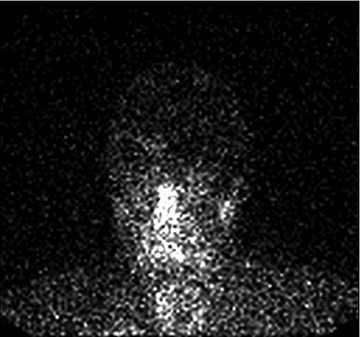
Fig. 3
One patient SPECT scan
1.2 Single Photon Emission Computed Tomography
SPECT scan uses a gamma camera that rotates around the patient to detect the radiotracer inside body. SPECT will also produce a set of 3D images but generally have a lower resolution. The radiotracers commonly used for SPECT scan include  [59],
[59],  [39],
[39],  [104],
  [23] etc. Electrocardiography (ECG)-Gated
  can also be used for myocardial perfusion PET [5]. One example image from SPECT scan is shown in Fig. 3. Hybrid SPECT/CT is also designed to provide more accurate anatomical and functional information [88]. SPECT scan differs from PET scan in that the tracer stays in your blood stream rather than being absorbed by surrounding tissues, therefore, SPECT scan can show how blood flows to the heart and brain are effective or not. SPECT scan is cheaper and more readily available than higher resolution PET scan. Tests have shown that SPECT scan might be more sensitive to brain injury than either MRI or CT scanning because it can detect reduced blood flow to injured sites. SPECT scan is also useful for presurgical evaluation of medically uncontrolled seizures and diagnosing stress fractures in the spine (spondylolysis), blood deprived (ischemic) areas of brain following a stroke, and tumors [4, 9].
[59], [39], [104], [23] etc. Electrocardiography (ECG)-Gated can also be used for myocardial perfusion PET [5]. One example image from SPECT scan is shown in Fig. 3. Hybrid SPECT/CT is also designed to provide more accurate anatomical and functional information [88]. SPECT scan differs from PET scan in that the tracer stays in your blood stream rather than being absorbed by surrounding tissues, therefore, SPECT scan can show how blood flows to the heart and brain are effective or not. SPECT scan is cheaper and more readily available than higher resolution PET scan. Tests have shown that SPECT scan might be more sensitive to brain injury than either MRI or CT scanning because it can detect reduced blood flow to injured sites. SPECT scan is also useful for presurgical evaluation of medically uncontrolled seizures and diagnosing stress fractures in the spine (spondylolysis), blood deprived (ischemic) areas of brain following a stroke, and tumors [4, 9].1.3 Other Molecular Imaging Modalities
Other molecular imaging modalities include MRI, CT, Optical imaging, Ultrasound, which have only limited molecular imaging abilities.
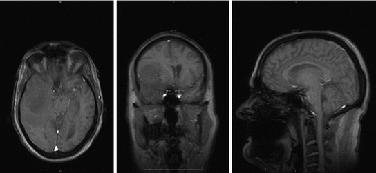
Fig. 4
One patient brain MRI scan
1.3.1 MRI
MRI scanners produce strong magnetic fields where body tissue that contains hydrogen atoms is made to emit a radio signal which is detected by the scanner. MRI scanners produce detailed 3D images of the inside of the body. MRI scan is best for brain imaging, breast, heart and blood vessel, organs and soft tissues [13]. Contrast materials are often used to enhance MRI images. MRI has the highest spatial resolution and possibility to extract both physiological and anatomical information. However, MRI generally has low sensitivity and requires longer scan and data processing time. Samples of MRI images are shown in Fig. 4.
Functional magnetic resonance imaging or functional MRI (fMRI) is a MRI procedure that measures brain activity by detecting associated changes in blood flow. The primary form of fMRI uses the blood-oxygen-level-dependent (BOLD) contrast, and measures the change in magnetization between oxygen-rich and oxygen-poor blood, which is mostly used in brain mapping research [37].
Another MRI scan used in research is Dynamic Contrast Enhanced- MRI (DCE-MRI), which is a quantitative method that allows for tumor vascular analysis, including blood volume, perfusion, vascular leakage space. DCE-MRI uses gadolinum-based contrast agents and standard MRI scanners to provide quantitative results [34].
1.3.2 Optical Imaging
Optical imaging has the highest sensitivity, but relatively low spatial resolution. Optical imaging only provides images in limited Field of View (FOV). Optical imaging reduces patient radiation exposed significantly by using non-ionizing radiation. Optical imaging can be used to differentiate between native soft tissues and tissues labeled with either endogenous or exogenous contrast media, using their different photon absorption or scattering profiles at different wavelengths. Optical imaging is also easy to be combined with other imaging modalities. In optical imaging, Diffusive Optical Imaging (DOI) is also known as Diffuse Optical Tomography (DOT) or Optical Diffusion Tomography (ODT). DOI is used to study the functions of brains, and can provide neural activities with its time courses [51]. Optical Coherence Tomography (OCT) produces 3D images from optical scattering media and penetrates biological tissues by using long wavelength light. OCT can provide higher SNR, faster signal acquisition [78].
1.3.3 Ultrasound
Ultrasound scanners emit high frequency sound and measure the reflected sound from the patients, which varies with the organs and tissues. Ultrasound imaging can be used to detect heart problems, examine liver, kidneys, abdomens, and guide a surgeon. Ultrasound can provide a real time imaging, but with limited spatial resolution. Most scans need targeted micro-bubbles to enhance the images [21].
Fig. 5
The whole procedure of PET data processing
2 The Challenges in Molecular Imaging Data Analysis
2.1 Data Processing for PET Imaging
The previous sections explain the advantages and limitations of molecular imaging modalities. Of all molecular imaging modalities, PET and SPECT are the full functional ones. Since PET and SPECT all belong to Emission Computed Tomography (ECT), many data correction and data analysis methods can be shared. In this section, we will focus on PET to demonstrate the challenges in data analysis. As shown in Fig. 5, the measurement data of PET is first stored in listmode. The listmode data can be corrected and reconstructed directly [66, 72], or rebinned by Fourier Rebinning to sinogram, which is corrected and reconstructed to be images [18]. The data correction process generally includes random correction, normalization, deadtime correction, attenuation correction and scatter correction. The corrected data will be reconstructed by either analytical or statistical algorithms to generate both activity images which are the concentrations of radiotracers in body and parametric images which are the dynamic changes of radiotracers represented by kinetic parameters.
The challenges in PET data analysis come from the change of statistical properties of measurement data after various data corrections. The quality of results from all image reconstruction algorithms depends on the accuracy of statistical models in each data correction and image reconstruction. However, due to the complexity of PET scan, it is nearly impossible to propose a perfect model. From next subsection, we will explain how the data corrections are applied and how they affect the data analysis.
2.1.1 Data Corrections
1.
Random Correction. Random coincidence events are two gamma photons from different positron annihilations are recorded as a Line of Response (LOR). The rate of random coincidences on a particular LOR is defined as  , where
  is the random coincident rate on the LOR connecting detector
  and
and  ,
,  is the coincidence timing window,
  and
and  are the singles rate on detector
  and
and  . The random coincidence rate depends on the detector circuit response, the most common method for estimating the random coincidence events is the delayed timing window method.
, where is the random coincident rate on the LOR connecting detector and , is the coincidence timing window, and are the singles rate on detector and . The random coincidence rate depends on the detector circuit response, the most common method for estimating the random coincidence events is the delayed timing window method.2.
Normalization. All the image processing methods assume the detector response are uniform and identical, however, in real clinical data acquisition, the performance of each detector will be different, the PMT gains are not exactly the same, and angle of incident of each gamma photon will also affect the detector sensitivity. The process of correcting these effects is normalization. One common clinical solution is to perform a scan using a uniform cylindrical phantom and a line source. In this scan, every possible LOR is illuminated by the same coincidence source.
3.
Deadtime Correction. The detector deadtime will cause the loss of coincidence events. Especially in the high count rate cases, the detector response will be significantly delayed due to the pile-up of incident gamma photons. A common solution is to model both paralyzable and non-paralyzable components from measurements of sources of different radioactivities.
4.
Attenuation Correction. Some gamma photons will be absorbed when interacting with the patients. The widely-adopted method for PET only scanner calculates the attenuation correction factors by using a rotating rod source with the object in the FOV. For hybrid PET/CT and PET/MRI scanners, the attenuation factors can be obtained by assigning predefined attenuation coefficients to the anatomical information generated by CT and MRI, which generally have a better spatial resolution.
5.
Scatter Correction. The coincidence events include those that the annihilation photons have an interaction of Compton scattering and change their directional and energy information before they arrive at the detector system. They are called scatter coincidences. Scatter coincidences will decrease the contrast, resolution and SNR of reconstructed images and need to be corrected properly. Scatter correction is the most complicated correction, we will use the scatter correction as an example to show how corrections affect the quantitative accuracy in PET scan.
2.1.2 Scatter Correction
Scatter Fraction. The scatter fraction is an important parameter included in both National Electrical Manufacturers Association (NEMA) and International Electrotechnical Commission (IEC) standards, and measured in every performance evaluation report of PET scanners. The scatter fractions of PET scanners from 3 major manufactures are listed in Table 1 [28, 40, 87].
Table 1
Scatter fractions of PET scanners from three main manufactures in 3D mode
Manufacture and model | Scatter fraction (%) |
|---|---|
Siemens TruePoint PET/CT | 32 |
GE discovery PET/CT | 33.9 |
Philips Gemini PET/CT | 27 |
Multiple Scatter Coincidence Events. The gamma photons can be scattered multiple times before recorded. Monte Carlo simulation is the best tool to study the Compton scattering during PET acquisition. We have done similar studies with our new PET scanner, HAMAMATSU SHR74000, we retrieve all the data, and analyze the composition of simulated measurement data according to the number of scattering of each photon in the coincidence photon pairs. The first data set is analyzed with the standard NEMA phantom, a 70 cm long, 20 cm diameter cylinder, the composition of scatter coincidences is summarized in Table 2. Furthermore, we have a lot of over-sized and over-weighted patients, especially in the western countries, and these patients usually take higher risk of many diseases than other patients. For these patients, their size makes more photons scattered inside their body, we correspondingly analyze the composition of scatter coincidence photons with a 70 cm long, 35 cm diameter cylinder, the results are summarized in Table 3. The number of total scatter coincidence events increase by about 20 %. If the tumor is near the body surface, the scatter fractions shown in Table 4 turn to be similar as in Table 2.
Table 2
The percentage of coincidence events assorted by the number of scattering of each photon
Photon2 \Photon1 | 0  (%) (%) | 1  (%) (%) | 2  (%) (%) | 3  (%) (%) | 4  (%) (%) |
|---|---|---|---|---|---|
0  | 55.36 | 16.58 | 1.92 | 0.11 | 0 |
1  | 16.56 | 5.81 | 0.68 | 0.04 | 0 |
2  | 1.92 | 0.7 | 0.08 | 0 | 0 |
3  | 0.11 | 0.04 | 0.005 | 0 | 0 |
4  | 0.005 | 0.001 | 0 | 0 | 0 |
Table 3
The percentage of coincidence events assorted by the number of scattering of each photon
Photon2 \Photon1 | 0  (%) (%) | 1  (%) (%) | 2  (%) (%) | 3  (%) (%) | 4  (%) (%) |
|---|---|---|---|---|---|
0  | 37.66 | 18.87 | 3.7 | 0.39 | 0.03 |
1  | 18.82 | 10.98 | 2.18 | 0.23 | 0.01 |
2  | 3.75 | 2.18 | 0.44 | 0.05 | 0 |
3  | 0.38 | 0.23 | 0.05 | 0.01 | 0 |
4  | 0.02 | 0.02 | 0 | 0 | 0 |
Table 4
The percentage of coincidence events assorted by the number of scattering of each photon
Photon2 \Photon1 | 0  (%) (%) | 1  (%) (%) | 2  (%) (%) | 3  (%) (%) | 4  (%) (%) |
|---|---|---|---|---|---|
0  | 59.23 | 16.28 | 2.94 | 0.38 | 0.03 |
1  | 16.29 | 1.18 | 0.1 | 0.01 | 0 |
2  | 2.94 | 0.1 | 0 | 0 | 0 |
3  | 0.38 | 0.01 | 0 | 0 | 0 |
4  | 0.04 | 0 | 0 | 0 | 0 |
Scatter Coincidence from Activity Concentrations outside of FOV. A whole body PET scan generally needs 4–5 bed positions to complete, then gamma photons from outside of FOV will also have the possibility to be misrecorded by the detector system. Sossi et al. show the scatter coincidence events need to be accounted for when the amount of radioactivity outside of FOV is comparable to the radioactivity inside the FOV in [81]. In the case of line sources, the scatter fraction increases by about 15 % when the source is extended 4 cm outside of the FOV and 20 % when it is extended 8 cm outside of the FOV. Spinks et al. also show for a full 3D PET, the scatter fraction increased from 40 to 45 % with the scatter photons from outside of FOV, after introducing a fitted brain shielding, the scatter fraction decreases to be 41 % [82]. A recent paper by Ibaraki et al. show the use of the neck-shield to suppress scatters from outside FOV can improve the SNR by 8 and 19 % for  and
and  , respectively [38].
and , respectively [38].Scatter Correction Methods. Bailey et al. [2] and Bentourkia et al. [7] present a Convolution-Subtraction (CS) scatter correction technique for 3D PET data. The scatter distribution is estimated by iteratively convolving the photo-peak projections with a mono-exponential kernel. The method is based on measuring the scatter fraction and the scatter function at different positions in a cylinder. The method performs well on 2D measurement data and also accounts for the 3D acquisition geometry and nature of scatter by performing the scatter estimation on 2D projections.
The method is easy to set up and still applies to a lot of animal studies, where the scatter correction are usually considered not necessary. Lubberink et al. propose a non-stationary CS scatter correction with a dual-exponential scatter kernel for scatter correction in both emission and transmission data of studies of conscious monkeys using Hamamatsu SHR7700 PET scanner [54] . Kitamura et al. implement a hybrid scatter correction method, which estimates scatter components with a dual energy acquisition using a CS to estimate the true coincidence events in the upper energy window for their four layer Depth of Interaction (DOI)—PET scanner [45]. Naidoo-Variawa et al. suggest that scatter correction methods based on spatially invariant scatter functions, such as CS, may be suitable for non-human primate brain imaging in [65].
Single Scatter Simulation (SSS) is one of the most important methods for PET scatter correction, and commercial PET scanners from Siemens are using SSS derived scatter correction methods. Ollinger [67] and Watson [98] first introduced the concept of model based scatter coincidence estimation. The single scatter approximation is defined with the well accepted formulation based on Klein-Nishina equation as
![$$\begin{aligned} S^{AB}=\int _v\left( \frac{\sigma _{AS}\sigma _{BS}}{4\pi R^2_{AS}R^2_{BS}}\right) \frac{\mu }{\sigma _c}\frac{d\sigma _c}{d\varOmega }[I_A+I_B], \end{aligned}$$](/wp-content/uploads/2016/10/A312883_1_En_2_Chapter_Equ1.gif)
where
 is the sampled scatter volume,
  is the scatter point,
  and
and  are sampled detectors, so
  is the coincidence scatter rate in detectors
  and
and  ,
,  and
and  are the detector cross sections presented to the rays
  and
and  ,
,  and
and  are the distances from
  to
to  and
and  .
.  and
and  are the total and differential Compton scattering cross sections,
  is the solid angle,
  is the energy of the non-scattered photon,
  is the energy of the scattered photon,
  and
and  are the approximated detector efficiencies for gamma rays which are incident along
  and
and  ,
,  is the linear attenuation coefficient at the energy
  and position
  , and
, and  is the estimated activity distribution from reconstructed images.
(1)
is the sampled scatter volume, is the scatter point, and are sampled detectors, so is the coincidence scatter rate in detectors and , and are the detector cross sections presented to the rays and , and are the distances from to and . and are the total and differential Compton scattering cross sections, is the solid angle, is the energy of the non-scattered photon, is the energy of the scattered photon, and are the approximated detector efficiencies for gamma rays which are incident along and , is the linear attenuation coefficient at the energy and position , and is the estimated activity distribution from reconstructed images.The calculation is repeated through all the sampled scatter points from activity distribution and sampled detector blocks. The final result is the distribution of single scatter coincidence events, and will be scaled and then subtracted from the measurement data to perform scatter correction. Figure 6 demonstrates the procedure of SSS based scatter correction for clinical PET scanner.
Fig. 6
The procedure of a SSS based scatter correction for clinical PET scanner
2.1.3 Dynamic PET Imaging
Dynamic PET imaging is a combination of short interval PET scans and reflects the dynamic metabolism of injected radiotracers. For example, a dynamic acquisition can consist of 85 frames in all: 15  0.2 min, 20
  0.5 min, 40
 1 min, and 10
  3 min. The series of acquisitions can be used to estimate the kinetic parameters which represent the metabolism of radiotracers in vivo. The difficulties in estimating kinetic parameters arise from the low count rates in the first several time frames and the low SNR. To obtain the kinetic parameters, a typical approach is first to reconstruct the activity distributions from the dynamic PET data, and then to fit the calculated time activity curve (TAC) to a predefined kinetic model. Samples of TAC curves in different organs are shown in Fig. 7. The accuracy of this kind of approaches relies on the reconstructed activity distributions. The complicated statistical noise properties, especially in the low-count dynamic PET imaging, and the uncertainties introduced by various PET data corrections will affect the activity reconstruction and lead to a suboptimal estimation of kinetic parameters [29]. There are also many efforts that try to estimate the kinetic parameters from PET projection data directly and achieve better bias and variance including both linear and nonlinear models [83, 91, 103]. One problem is that the optimization algorithms are very complicated. Kamasak et al. apply the coordinate descent algorithm for optimization but it is still limited to specific kinetic models [61]. Wang et al. apply a generalized algorithm for reconstruction of parametric images [96], however, it still lacks of estimation and analysis of individual kinetic parameter. Exactly, every kinetic parameter has its own physical meaning like radiotracer transport rate, phosphorylation rate and dephosphorylation rate (it is very sensitive to the system [35]) in FDG study, which will be critical to clinical research, drug discovery and drug development [15, 92].
0.2 min, 20 0.5 min, 40 1 min, and 10 3 min. The series of acquisitions can be used to estimate the kinetic parameters which represent the metabolism of radiotracers in vivo. The difficulties in estimating kinetic parameters arise from the low count rates in the first several time frames and the low SNR. To obtain the kinetic parameters, a typical approach is first to reconstruct the activity distributions from the dynamic PET data, and then to fit the calculated time activity curve (TAC) to a predefined kinetic model. Samples of TAC curves in different organs are shown in Fig. 7. The accuracy of this kind of approaches relies on the reconstructed activity distributions. The complicated statistical noise properties, especially in the low-count dynamic PET imaging, and the uncertainties introduced by various PET data corrections will affect the activity reconstruction and lead to a suboptimal estimation of kinetic parameters [29]. There are also many efforts that try to estimate the kinetic parameters from PET projection data directly and achieve better bias and variance including both linear and nonlinear models [83, 91, 103]. One problem is that the optimization algorithms are very complicated. Kamasak et al. apply the coordinate descent algorithm for optimization but it is still limited to specific kinetic models [61]. Wang et al. apply a generalized algorithm for reconstruction of parametric images [96], however, it still lacks of estimation and analysis of individual kinetic parameter. Exactly, every kinetic parameter has its own physical meaning like radiotracer transport rate, phosphorylation rate and dephosphorylation rate (it is very sensitive to the system [35]) in FDG study, which will be critical to clinical research, drug discovery and drug development [15, 92].Fig. 7
a Standard zubal phantom; b TAC curves of three ROIs indicated in (a); c sample TAC curves of true lesion and false lesion
3 General Framework of Shape Analysis in Molecular Imaging
3.1 Image Segmentation
In computer vision, image segmentation is the process of partitioning an image into multiple different segments (group of pixels). Especially in molecular imaging, the image segmentation is used to simplify the representation of an image and extract Region of Interest (ROI) that is more meaningful and followed by image analysis. Image segmentation is also important to find the boundaries of different regions and organs by applying different labels. Image segmentation can also be applied to 3D image stacks to help 3D image reconstruction [17, 106].
The aforementioned limitations of PET and SPECT also bring new challenges to image segmentation. Here we will introduce several basic image segmentation methods.
1.
2.
Cluster based method is a multivariate data analysis method that uses predefined criteria to partition a large number of objects into a smaller number of clusters, in which the objects are similar to each other. Cluster based method has been applied to fMRI imaging and then dynamic PET imaging, with limited spatial resolution and SNR [101].
3.
Gradient based method is to find the boundary of an object of interest with the gradient intensity observed in the image. This kind of method is fast and easy to apply, but generally works together with other method to achieve better results in molecular imaging [26].
4.
Level set based method derives from snake method (active contour model), which delineates an object outline from a noisy image by attempting to minimize an energy associated to the contour as a sum of internal and external energies [57, 68]. Many methods are derived from basic level set method including deformable level set models, which have the ability to automatically handle topology [33], 3D level set methods to compute 3D contours [105] etc.
3.2 Image Registration
Image registration is the process to transform different sets of data into one coordinate system. Image registration is widely used in molecular imaging, e.g. patient radiotherapy follow-up by transforming PET images from a series of studies, diagnosis by images from multiple imaging modalities [16, 32, 36, 75]. With the development of hybrid PET/CT, PET/MRI, the image registration with multiple images in one study is made easier because the motions of patients are minimized by the simultaneous data acquisition. However, images from multiple studies still need good image registrations. Mainstream image registration methods for molecular imaging include
1.
Intense-base image registration. Since PET and SPECT imaging reflects the concentrations of radiotracer, intense based methods compare intensity patterns in multiple images and register the reference image and target image by defining correlation metrics [46].
2.
3.
Multiple modality image registration. The hybrid PET/CT and PET/MRI make the image registration focus on the deformations from patients’ respirations and motions [27, 60]. The image registration can be improved by different patient preparation and pre-positioning [8], respiratory gating [10], various tracking devices etc. [76].
3.3 Image Fusion
Image fusion is the combination of relevant information from two or more images into one single image. The fused image will provide more information than any single input image. Accurate image fusion from combined PET, CT, MRI scans can significantly improve the diagnosis and provide better understandings of diseases. Image fusion generally works together and shares similar technologies with image registration [69, 89, 95].
3.4 Image Reconstruction
Image reconstruction is the process to reconstruct 2D and 3D images from acquisition data of molecular imaging modalities. Reconstruction algorithms include both analytical ones, e.g. Filtered Back Projection (FBP) and iterative ones, e.g. Maximum Likelihood (ML). Analytical algorithms are computationally fast, especially when applied to full 3D image reconstruction using 3D-FBP. FBP is also used in dynamic PET image reconstruction, where it is believed to provide better quantitative accuracy with the extremely low count data sets. Iterative algorithms are currently the mainstream reconstruction algorithms, which use statistical assumptions and provide images of overall better qualities. Image reconstruction is one of the most important processes in data processing, other image-based processes and clinical diagnosis all depend on the accuracy of reconstructed images.
3.5 Dynamic PET Analysis
3.5.1 Clinical Requirements
The accuracy of quantitative dynamic PET studies depends on various factors including kinetic models, quantitative methods and the approximation of arterial input function from blood sampling. The most general kinetic models used are compartment model with assumptions that physiological process and molecular interactions are not influenced by injected radioligand. Current clinical adopted quantitative methods are actually semi-quantitative methods, which include methods using reference regions or calculating Standard Uptake Value (SUV). Methods using reference regions are easy to implement but have several drawbacks, e.g. the reference tissue is hard to define and has low SNR due to the low resolution of PET and SPECT scans, and the uptake of the reference tissue may change after the radiotherapy. SUV now is included in every clinical study, which is calculated as a ratio of tissue radioactivity concentration and injected dose divided by body weight, the advantage of SUV in clinical study is that the blood sampling is not required. However, the full quantitative analysis requires both dynamic PET scans and tracer concentration in the arterial blood plasma. The gold standard of blood sampling is serial arterial sampling of a superficial artery, and clinical alternative methods include venous blood sampling, image derived input function and population based input function. The drawback of the full quantitative method is only one FOV/bed position can be taken into consideration. For metastasized disease, not all lesions can be quantified simultaneously.
Fig. 8
Illustration of six basic compartment models
3.5.2 Compartment Models
Compartment models are used in many fields including pharmacokinetics, biology, engineering etc. Compartment models are the type of mathematical models to describe the way materials (radiotracers and their metabolite in PET and SPECT scan) are transmitted among the compartments (different organs and tissues). Inside each compartment, the concentration of radiotracers is assumed to be uniformly equal. Due to their simplicity and plausibility, compartment models are widely used in the dynamic PET scans to describe the tracer/drug kinetics.
Drug kinetic models include simple drug transport model, which generally contains equal or less than three compartments and can be solved directly, and complicated biological models, which can contain up to twenty compartments and generally require prior knowledge to solve [30, 31]. Most of the complicated models with many compartments can usually be decomposed into a combination of simple models with less than four compartments. The most basic compartment models used in kinetic analysis shown in Fig. 8 include two compartment blood flow model (Model 1), standard two tissue three compartment Phelps 4K model with reversible target tissue (Model 2) and Sokoloff 3K model with irreversible target tissue (Model 3), three tissue five parameter bertoldo model (Model 4), standard three tissue four compartment model (Model 5 and Model 6). More complicated models with more compartments and parallel model with multiple injection can be extended from aforementioned standard models [24, 44].
All six models can be represented by a set of differential equations with corresponding kinetic parameters K =  , where
  is the number of kinetic parameters. Here we utilize Model 2 as an example for demonstration. Model 2 can be represented by first-order differential equations
The measurement of dPET is the combination of radiotracer in plasma  , non-specific binded radiotracer
  and specific binded radiotracer
  through
where  is the blood volume fraction, Y is measured projection data , D is the system probability matrix, and
  is the noises during acquisition. Equation (5) can be represented by a more general time-dependent form for all models as
Simple models with less than three compartments generally can be solved directly, while more complicated models need simplifications and various numerical approximations.
, where is the number of kinetic parameters. Here we utilize Model 2 as an example for demonstration. Model 2 can be represented by first-order differential equations(2)
(3)
, non-specific binded radiotracer and specific binded radiotracer through(4)
(5)
is the blood volume fraction, Y is measured projection data , D is the system probability matrix, and is the noises during acquisition. Equation (5) can be represented by a more general time-dependent form for all models as(6)
4 Review of Recent Advancements of Shape Analysis
4.1 Mathematical Modeling and Statistical Formulation of PET Image Reconstruction
4.1.1 Statistical Image Reconstruction Criterion
The goal of mathematical modeling of data acquisition is to describe the transforms from spatial distribution of imaging objects to projection distributions on detector pairs in PET system. Denoting the spatial distribution of imaging object by a set of spatial variables  , where
  is the total number of voxels, and the expected values (means) of projection bins by
  , where
  is the total number of bins, a mathematical expression of the transform can be obtained

where  is the system response model giving the probability matrix of mapping the transform from
  to
to  , and
, and  is the means of background noises. A block diagram of the above procedure is shown in Fig. 9a.
, where is the total number of voxels, and the expected values (means) of projection bins by , where is the total number of bins, a mathematical expression of the transform can be obtained(7)
is the system response model giving the probability matrix of mapping the transform from to , and is the means of background noises. A block diagram of the above procedure is shown in Fig. 9a.With the mathematical model specified above, the problem of PET image reconstruction is to find an estimation of the imaging object  from the measurement data (projection bins)
  . The image reconstruction is an ill-posed inverse problem, so an intuitive solution is to apply statistical assumptions of measurement data as regularizations. The statistical formulation tries to find an optimized relationship between measurement data
  and imaging object
  (or expected values of projection bins
  ) by defining different objective functions. If denoting
  is the measurement data
  after all data corrections and assuming all the data correction are perfectly applied,
  is equal to the
  after all data corrections, however, in real clinical data acquisition, there will be some difference between
  and
and  , which is accumulated from residuals of each data correction.
from the measurement data (projection bins) . The image reconstruction is an ill-posed inverse problem, so an intuitive solution is to apply statistical assumptions of measurement data as regularizations. The statistical formulation tries to find an optimized relationship between measurement data and imaging object (or expected values of projection bins ) by defining different objective functions. If denoting is the measurement data after all data corrections and assuming all the data correction are perfectly applied, is equal to the after all data corrections, however, in real clinical data acquisition, there will be some difference between and , which is accumulated from residuals of each data correction.Fig. 9
Block diagrams. a PET data acquisition; b Statistical model based iterative PET reconstruction; c Designed system for PET image reconstruction; d Simplified block diagram (black box) of (c)
A block diagram of statistical image reconstruction framework is shown in Fig. 9b: the statistical properties of system noises or measurement data are first modeled based on certain statistical distributions (Gaussian, Poisson, their combination or other derivations) in block  , then inputted into system block
  ; the system output is generated and compared with corrected measurement data
  based on the predefined criteria, when the system goes convergent, estimations of the imaging object
  will be obtained. Three major criteria can be used are Least Square based (LS), Maximum Likelihood based (ML), Maximum A Posterior based (MAP).
, then inputted into system block ; the system output is generated and compared with corrected measurement data based on the predefined criteria, when the system goes convergent, estimations of the imaging object will be obtained. Three major criteria can be used are Least Square based (LS), Maximum Likelihood based (ML), Maximum A Posterior based (MAP).LS based methods try to obtain the estimation  by minimizing the difference of fit between the predicted data by means of the modeling of the acquisition process and the measured data
  , the general objective function is
Extended algorithms are all based on the above equation and try to improve the performance by introducing different weights or penalization items.
by minimizing the difference of fit between the predicted data by means of the modeling of the acquisition process and the measured data , the general objective function is(8)
ML based methods try to obtain the estimation  by maximizing the likelihood functions which represent the goodness of fitting statistical assumptions to measurement data. The general objective function is based on the conditional probability density of the image object with known measurement data
  as
as
where  represents the probability density, and the above equation is a function of
  . When a statistical model of measurement data or noises is defined, either Gaussian/Poisson or their combination, the objective likelihood function can be solved correspondingly. An improved method based on poisson assumption widely used is EM-SP (Shifted Possion) algorithm, which introduces two times the mean of randoms coincidences to the random precorrected data and models this sum as a Poisson random variable, and the objective function is still based on the above one [63]. Furthermore, a priori information can also be introduced in the form of statistical properties of the imaging object as constraints into the ML objective function.
by maximizing the likelihood functions which represent the goodness of fitting statistical assumptions to measurement data. The general objective function is based on the conditional probability density of the image object with known measurement data as(9)
represents the probability density, and the above equation is a function of . When a statistical model of measurement data or noises is defined, either Gaussian/Poisson or their combination, the objective likelihood function can be solved correspondingly. An improved method based on poisson assumption widely used is EM-SP (Shifted Possion) algorithm, which introduces two times the mean of randoms coincidences to the random precorrected data and models this sum as a Poisson random variable, and the objective function is still based on the above one [63]. Furthermore, a priori information can also be introduced in the form of statistical properties of the imaging object as constraints into the ML objective function.Bayesian formulation is such a probabilistic approach, statistical information of the unknown imaging object  is introduced by adopting the probability density of
  , which is the prior
  . Equation (9) can then be solved as follow:
is introduced by adopting the probability density of , which is the prior . Equation (9) can then be solved as follow: