of a vertebra with one genus is represented by triangular patches. For each vertex 
 in
in  , its 1-ring region
  consists of
  patches containing the vertex
  .
.
2.1 Modified Self-organizing Deformable Model
The mSDM is a deformable model whose shape is deformed by using a competitive learning and an energy minimization approach. Regrading a tissue model as the mSDM, the model is mapped onto a target surface by fitting the model to the target surface. The overview of the mSDM algorithm is as follows.
Step. M-1
A vertebra model  is deformed to fit to the target surface by the original SDM algorithm [9].
 is deformed to fit to the target surface by the original SDM algorithm [9].
Step. M-2
The deformed model may contain foldovers. To realize the one-to-one correspondence, the foldover is removed by moving the vertices to within their 1-ring region.
Step. M-3
After the Step. M-2, the feature vertices move away from their corresponding points. Free-Form Deformation (FFD) [10] is applied to the mapped model to correct the positions of the feature vertices.
Step. M-4
To compare with the models, it is desirable that the mapped model preserves the original geometric properties as far as possible. Such deformation is achieved by an area- and/or angle-preserving mapping  . Practically, the model obtained after Step. M-3 is deformed by minimizing an objective function
  that is a weighted linear combination of area error term
  and angle error term
  :
:


where  is a scaling factor to adjust the ranges of the two error terms.
  and
and  are the area and one angle of the patch
  included in the 1-ring region
  of the vertex
  .
.  and
and  is the area and angle of the patch in
  . The area errors in Eq. (3) is obtained by the total difference between the area ratio of a patch before and after the mapping. Here, the area ratio of the patch
  is defined as the ratio of the area
  of
of  to the whole area of the 1-ring region
  of
of  . In the same way, the angle error in Eq. (4) is obtained by the total difference between the angles of the patch
  before and after the mapping. Changing the weighting factor
  from 0 to 1, the mapping becomes from angle- to area-preserving mapping. The setting of
  determines the kinds of geometrical features preserved after the mapping. The discussion about the setting of
  will be found in [1]. From Eqs. (1) and (2), the minimization of Eq. (1) is replaced as the optimization problem of positioning the vertices in the 1-ring region by moving them repeatedly. The optimal mapping is found by applying a greedy algorithm with Eq. (2). Then, the vertices are not on the target surface completely. Therefore, they are mapped onto the nearest patch of the target surface after the movement.
 . Practically, the model obtained after Step. M-3 is deformed by minimizing an objective function
  that is a weighted linear combination of area error term
  and angle error term
  :
:
(1)

(2)

(3)

(4)
 is a scaling factor to adjust the ranges of the two error terms.
  and
and  are the area and one angle of the patch
  included in the 1-ring region
  of the vertex
  .
.  and
and  is the area and angle of the patch in
  . The area errors in Eq. (3) is obtained by the total difference between the area ratio of a patch before and after the mapping. Here, the area ratio of the patch
  is defined as the ratio of the area
  of
of  to the whole area of the 1-ring region
  of
of  . In the same way, the angle error in Eq. (4) is obtained by the total difference between the angles of the patch
  before and after the mapping. Changing the weighting factor
  from 0 to 1, the mapping becomes from angle- to area-preserving mapping. The setting of
  determines the kinds of geometrical features preserved after the mapping. The discussion about the setting of
  will be found in [1]. From Eqs. (1) and (2), the minimization of Eq. (1) is replaced as the optimization problem of positioning the vertices in the 1-ring region by moving them repeatedly. The optimal mapping is found by applying a greedy algorithm with Eq. (2). Then, the vertices are not on the target surface completely. Therefore, they are mapped onto the nearest patch of the target surface after the movement.
Once a tissue model and its target surface are given, our mSDM is performed automatically with no users’ manual intervention. Moreover, the mSDM framework controls the movement of several feature vertices of the model. Practically, when users manually specify the feature vertices and their corresponding locations on the target surface, the SDM algorithm maps the tissue model onto the target surface while moving the feature vertices toward their corresponding locations. This characteristic of the mSDM makes it easy to find the correspondence between tissue models by mapping the anatomical feature vertices of the tissue model onto their specific locations on the target surface.
2.2 Vertebra Parameterization Using mSDM
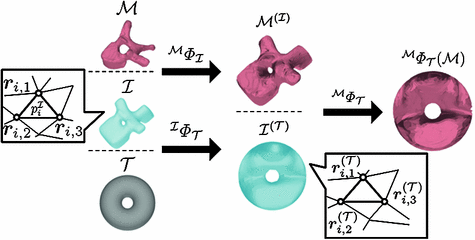
Our parameterization method uses an intermediate surface  whose shape is close to vertebrae shape. Here, the intermediate surface is determined as a surface model which has intermediate shape between the vertebra and the torus. Figure 1 shows the overview of the mapping a vertebra
  onto a torus
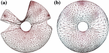
  . When the vertebra is mapped directly onto the torus whose shape is far from the vertebra, users need to tune the parameters in the mSDM algorithm and the scale of the torus. Especially, the latter tuning is to change the size of the torus and its hole according to the hole size of each individual vertebra. If the user fails the initial settings, we sometimes obtain the incomplete one-to-one mapping between the vertebra and the torus. Figure 2a, b show the examples of the vertebra models obtained by mapping the vertebra onto the torus directly. As shown in Fig. 2, the accuracy of the direct mapping depends on the parameters and the scale tuning heavily. On the other hand, through our experiments, the use of the intermediate surface results in the stable mapping of the vertebra models independent of the tuning for individual models. At first, we find one-to-one mapping
  between
  and
and  . Similarly, one-to-one mapping
  from
from  to
to  is found. Combining the two mappings
  and
and  , we obtain the mapping
  from
from  to
to  .
.
 whose shape is close to vertebrae shape. Here, the intermediate surface is determined as a surface model which has intermediate shape between the vertebra and the torus. Figure 1 shows the overview of the mapping a vertebra
  onto a torus
  . When the vertebra is mapped directly onto the torus whose shape is far from the vertebra, users need to tune the parameters in the mSDM algorithm and the scale of the torus. Especially, the latter tuning is to change the size of the torus and its hole according to the hole size of each individual vertebra. If the user fails the initial settings, we sometimes obtain the incomplete one-to-one mapping between the vertebra and the torus. Figure 2a, b show the examples of the vertebra models obtained by mapping the vertebra onto the torus directly. As shown in Fig. 2, the accuracy of the direct mapping depends on the parameters and the scale tuning heavily. On the other hand, through our experiments, the use of the intermediate surface results in the stable mapping of the vertebra models independent of the tuning for individual models. At first, we find one-to-one mapping
  between
  and
and  . Similarly, one-to-one mapping
  from
from  to
to  is found. Combining the two mappings
  and
and  , we obtain the mapping
  from
from  to
to  .
.
Fig. 1
Vertebra parameterization using mSDM

Fig. 2
Mapped vertebra models onto the torus by applying direct mapping a before and b after parameter and scale tuning of the SDM and the torus
Our parameterization method consists of four steps.
Step. P-1
Select an intermediate surface  .
.
 .
.Step. P-2
Find a mapping  by mapping from
  to
to  with mSDM.
 by mapping from
  to
to  with mSDM.
Step. P-3
Find a mapping  by mapping from
  to
to  with mSDM.
 by mapping from
  to
to  with mSDM.
Step. P-4
Obtain the direct mapping  by combining
  and
and  .
.
 by combining
  and
and  .
.The following describes the detail of Step. P-4. Let us denote as  the model
  mapped onto the intermediate surface
  . For each vertex
  in
in  , we find a closest patch
  in
in  to the vertex
  . When,
  consists of three vertices
  (Fig. 1), the coordinate of
  is represented by

where  and
and  (
( ) are real number parameters. Similarly, using the mapping
  , the vertices
  in
in  are represented by
  . Therefore, the vertices
  of the model mapped on the torus are obtained by replacing the coordinates of vertices in
  with that in
  in Eq. (5):
 the model
  mapped onto the intermediate surface
  . For each vertex
  in
in  , we find a closest patch
  in
in  to the vertex
  . When,
  consists of three vertices
  (Fig. 1), the coordinate of
  is represented by
(5)
 and
and  (
( ) are real number parameters. Similarly, using the mapping
  , the vertices
  in
in  are represented by
  . Therefore, the vertices
  of the model mapped on the torus are obtained by replacing the coordinates of vertices in
  with that in
  in Eq. (5):

