and Diffusion Tensor Imaging: Applications in Skeletal Muscles

Fig. 1

This figure shows the arrangement of the muscle fibers as well as the connective tissue (endomysium, perimysium, and epimysium) surrounding the muscle fiber, bundles of muscle fiber, and the whole muscle compartment, respectively. Diffusion anisotropy can be understood in the context of the muscle fiber arrangement [Reprinted from SEER training modules, ‘Structure of Skeletal Muscle’. U.S. National Institutes of Health, National Cancer Institute. 02-09-2013 (date of access), http://training.seer.cancer.gov/anatomy/muscular/structure.html]

4 Imaging Pulse Sequences for Diffusion-Weighted Magnetic Resonance Imaging

The pulse sequences used to measure the diffusion tensor in muscle are similar to those implemented for the brain (Basser and Jones 2002). They are based on the spin echo, echo planar diffusion-weighted sequence. It should be noted that muscle imaging is challenged by the following characteristics of muscle: low T2 (32 ms for muscle compared to 70–80 ms for brain tissue), low FA (0.2–0.3 for muscle compared to 0.4–0.8 for white matter), and fat infiltration in the muscle (admixture of fat and muscle in a voxel). These considerations have led to sequences with a short TE and efficient fat suppression methods. Approaches to increase SNR include larger voxel sizes, increased averages, and the use of surface coils.

4.1 Spin Echo, Echo Planar Diffusion-Weighted Imaging

The basic physics behind obtaining diffusion-weighted MR images involves the use of two large balanced diffusion gradient sequences, placed around the 180° refocusing pulse (Fig. 2). The first gradient introduces a dephasing of spins that is determined by the magnitude, G, and duration, δ, of the diffusion gradient. The second gradient will completely rephase the phase introduced by the first gradient if the spins are entirely static. The large diffusion gradients and long duration, however, affect the signal from molecules undergoing motion, even on the scale of diffusion-related displacements. Since the sequence is sensitive to these small motions, it is important to acquire the image in very short times in order to freeze all physiological and other motion. This is achieved using an echo planar readout which can acquire a 2D image in ~40–100 ms (echo planar readout not shown in the figure).

Fig. 2

Diffusion gradient sensitization with a spin echo preparation, the echo planar readout is not shown here. The top pulse sequence (a) is used for the baseline acquisition (without diffusion preparation) and the bottom pulse sequence (b) includes the diffusion gradient lobes (G) which can be applied along any direction

The effect of the two diffusion gradient lobes (strength, duration, and diffusion time) is represented by a single term called the “b-factor” defined as (Basser and Jones 2002):

$b = \gamma^{2} G^{2} \delta^{2} \left( {\Updelta - {\raise0.7ex\hbox{$\delta $} \!\mathord{\left/ {\vphantom {\delta 3}}\right.\kern-0pt} \!\lower0.7ex\hbox{$3$}}} \right)$

where the gradient parameters are defined in Fig. 2.

The signal intensity of a diffusion-weighted image, S(b) with respect to the baseline image (all parameters the same but without the diffusion gradient) for the general case of anisotropic diffusion is given by (Basser and Jones 2002):

$\begin{aligned} & { \ln }\left( {\frac{S\left( b \right)}{{S\left( {b = 0} \right)}}} \right) = - \sum\limits_{i = 1}^{3} {\sum\limits_{j = 1}^{3} {b_{ij} } } D_{ij} \\ & = - \left( {b_{xx} D_{xx} + 2b_{xy} D_{xy} + 2b_{xz} D_{xz} + b_{yy} D_{yy} + 2b_{xz} D_{xz} + b_{zz} D_{zz} } \right) \\ \end{aligned}$

In order to extract the six components, D _ij, of the diffusion tensor, diffusion gradients have to be applied in at least six noncollinear directions. When using greater than six directions for the diffusion gradients, there is a tradeoff between number of averages and diffusion gradient directions. The diffusion tensor is diagonalized to obtain the eigenvalues (λ ₁, λ ₂, λ ₃) and eigenvectors (ν ₁, ν ₂, ν ₃) of the diffusion tensor ellipsoid. The eigenvector corresponding to the largest eigenvalue has been validated to be along the fiber directions. The eigenvectors define the orientation of the anisotropic diffusion ellipsoid, while the degree of anisotropy is defined by the relative magnitude of the eigenvalues. The “mean diffusivity,” MD, alternately termed as the “apparent diffusion coefficient, ADC,” is the average of the three eigenvalues:

${\text{MD}} = \frac{{\lambda_{1} + \lambda_{2} + \lambda_{3} }}{3}$

FA is a scalar measure of this anisotropy and is derived from the eigenvalues as:

${\text{FA}} = \sqrt\frac{2}{3} \sqrt{\left( {\frac{{\left( {\lambda_{1} - \lambda_{\text{av}} } \right)^{2} + \left( {\lambda_{2} - \lambda_{\text{av}} } \right)^{2} + \left( {\lambda_{3} - \lambda_{\text{av}} } \right)^{2} }}{{\lambda_{1}^{2} + \lambda_{2}^{2} + \lambda_{3}^{2} }}} \right)}$

FA values range from 0 (isotropic) to 1 (strongly anisotropic). The FA values in muscle are in the range of 0.2–0.3 which is lower than that of white matter (~0.5–0.8). Besides the mean diffusivity and the FA, several scalar measures derived from the tensor have been proposed. These include other measures of anisotropy like the shape of the diffusion: whether it is like a cigar (linear), pancake (planar), or sphere (spherical) (O’Donnell and Westin 2011).

The eigenvectors are conveniently represented in color and the following conventions are used in DTI visualization: with the x-projections mapped to red, y-projections to green, and z-projections to blue. The ultimate goal is to obtain the fiber tracks which represent the physiological unit of the muscle fiber bundles. Several tractography algorithms have been proposed to connect eigenvectors; the most commonly used is known as fiber assignment by continuous tracking, FACT (Mori and van Zijl 2002; O’Donnell and Westin 2011). In this algorithm, the algorithm starts from seed voxels defined by the user or by FA thresholds and follows the eigenvector direction in each voxel. Termination occurs when the FA value falls below a preset threshold or the orientation of the fiber changes by a larger angular threshold. Tract selection (using anatomical ROIs) and seed placement are highly interactive resulting in a strong operator dependence of fiber tracts. Another related approach is streamline tractography which also works by successively stepping in the direction of the principal eigenvector. Several computational methods are used to perform basic streamline tractography: Euler’s method (following the eigenvector or tangent for a fixed step size) and second order or fourth order Runge–Kutta method (where the weighted average of two or four points is used for each successive step) (Basser et al. 2000). More advanced methods in tractography include probabilistic tractography that provides a measure of the probabilities of connections (Behrens et al. 2003) and tractography using advanced models for fiber crossings (Malcolm et al. 2010). Tractography is an area of active research and a recent review comparing different tractography algorithms is discussed by Lazar (2010). In muscle fiber tracking, FACT and streamline tractography methods have been used in almost all the studies reported so far. Muscle fibers do not cross and present simpler geometrical constructs compared to brain white matter fibers may be one of the reasons for the success of the simpler deterministic algorithms. However, as seen later, muscle tractography is still challenged by the lower FA values, lower SNR as well as the admixture of fat in muscle voxels.

4.1.1 Simulation Studies

Simulation studies have been performed incorporating low T2 values, % muscle fraction, DTI indices (eigenvalues, and FA) typical values for muscle in order to obtain the optimum acquisition parameters and SNR requirements to measure DTI indices with a given accuracy (Damon 2008). In the latter paper, simulations were performed with six standard diffusion gradient directions, and identified the optimum b value to be between 400 and 700 mm²/s, and SNR of 25 for the baseline image was required to obtain an accuracy of 5 % in the DTI indices when the voxel contained only muscle tissue. The SNR requirements for eigenvector directions were more stringent: SNR ≥25 and ≥45 was required for eigenvector angular deviations of ±4.5° uncertainty with muscle fractions of 1 and 0.5, respectively. When considering single voxel angular uncertainty, and SNR ≥60 was required for ±9° uncertainty; this can have consequences for accurate fiber tracking. Froeling also performed simulation studies and determined that at least 12 gradient directions should be employed (Froeling 2012). Increasing the number of gradient directions does increase the accuracy of the eigenvector but it should be balanced by the number of averages so that the acquired diffusion-weighted images are of sufficient image quality to permit image preprocessing (for distortion corrections etc.). A more recent study also considered the effect of fat infiltration/admixture in the muscle and showed that regions must contain at least 76 % muscle tissue to reflect the diffusion properties of pure muscle accurately (Williams et al. 2013). In fat-suppressed diffusion-weighted images, high values of FA were surprisingly found in regions with high % of fat. This was attributed to the lower SNR in these regions which biased the value of the FA. This type of FA bias has been shown in earlier simulation studies focused on the brain as well (Basser and Pajevicz 2000).

It should be noted that the optimum b-value for diffusion imaging (~400 s/mm²) is lower than that used in the brain (~1,000 s/mm²). This allows lower TE values for the sequence which addresses the lower T2 of the muscle. Saupe et al. determined the optimum b-value at 1.5 T for muscle imaging using fiber tracking quality for evaluation; they estimated the optimum value to be 625 s/mm² (Saupe et al. 2009). Another important aspect is that most of the DWI/DTI sequences for the brain use a dual 180° pulse (twice refocused) to reduce the effects of eddy current. Most of the muscle DWI/DTI studies reported so far do not use the twice refocused for eddy current correction in order to keep TE at a minimum value. Further, it should be noted that the lower ‘b’ values used in muscle DTI do not result in large eddy current artifacts and the smaller eddy current distortions are corrected using post-processing methods.

Typical parameters and scan settings used in spin-echo echo-planar imaging (SE-EPI) based DTI acquisition for the lower leg calf muscles are listed below (Sinha et al. 2011). The acquisition included one baseline and 13 diffusion-weighted images (b factor: 500 s/mm²) along 13 noncollinear gradient directions. Image acquisition parameters were as follows: Echo Time (TE)/Repetition Time (TR)/Field-of-View (FOV)/matrix: 48 ms/6,400 ms/24 cm/128 × 128 with parallel imaging. Images were reconstructed to a matrix size of 256 × 256; voxel resolution was 0.94 × 0.94 mm in-plane resolution (after reconstruction to a 256 × 256 matrix) with a slice thickness of 5 mm. The sensitivity encoding (SENSE) method was employed in the parallel image reconstruction and a reference scan for coil sensitivity calculation was acquired prior to each DTI acquisition; a parallel imaging reduction factor of two was used. The volume of interest was also shimmed prior to the DTI acquisition. A total of 29–30 slices were acquired contiguously, and six repeats of the acquisition were magnitude averaged for a total scan time of 9 min. A spatial spectral fat-saturation pulse was used to suppress the fat signal.

4.2 Stimulated-Echo Planar Diffusion-Weighted Imaging

The overwhelming number of muscle DTI studies have used the spin echo EPI diffusion-weighted imaging. A few studies, however, have used the stimulated echo sequence since it permits diffusion weighting at small values of TE; as explained earlier, the latter is advantageous since muscle T2 is low. In this method, three 90° pulses are applied: the first diffusion lobe is applied between the first two 90° pulses and the balancing diffusion gradient is applied after the third 90° pulse (Fig. 3). The time between the second and third 90° pulse (~the diffusion time) can be fairly long as the magnetization is stored longitudinally (Fig. 3). Thus for the same ‘b’ value in SE and STE, the gradient strength and duration can be smaller since the diffusion time, delta, can be made fairly large. The TE of the STE sequence depends on the time between the first two 90° pulses: this can be made much smaller than the SE analog. However, the SNR of the STE signal is reduced by half compared to an SE signal and this affects the overall image quality. Schwenzer et al. studied the variation of muscle diffusion indices with flexion using an STE-EPI sequence (Schwenzer et al. 2009). More recently, Karampinos et al. combined eddy-current compensated diffusion-weighted stimulated-echo preparation with sensitivity encoding (SENSE, reduction factor 2.86) to obtain high SNR and to reduce the sensitivity to distortions and T(2)* blurring in high-resolution skeletal muscle single-shot DW-EPI (Karampinos et al. 2012). The rather high reduction factor of 2.86 certainly reduced distortions and fat–water mismapping artifacts, but also contributes to a loss in SNR. They were able to obtain voxel resolutions of 17 mm³ which is of the order achievable with single-shot SE-EPI DW imaging. The TE (31 ms) is lower than that possible with SE-EPI (~42–49 ms) but is still not low enough to compensate for the loss in signal intensity by a factor of 0.5 in a STEAM acquisition. The few studies, so far, have not convincingly demonstrated that STE diffusion preparation offers a distinct advantage over the SE diffusion preparation (note: parallel imaging has been used with both techniques to reduce the distortion/fat mismapping artifacts). A recent clinical study uses STE diffusion preparation to study Chronic Exertional Compartment Syndrome (CECS) of the Lower Leg Muscles (Sigmund et al. 2013).

Fig. 3

Schematic of eddy-current compensated stimulated-echo prepared DW-EPU pulse sequence. Diffusion weighting gradients are in black and eddy current compensating gradients are in gray [Reprinted with permission from Karampinos et al. (2012)]

5 Post-processing of Diffusion-Weighted Images

Echo planar diffusion-weighted images suffer from low signal-to-noise and from geometric distortion artifacts arising from eddy currents as well as from B0 field inhomogeneities. Several groups have adapted denoising and correction techniques originally developed for brain images to muscle DTI data.

5.1 Denoising

Froeling et al. have used a Rician linear minimum mean square error (LMMSE) noise suppression algorithm on the diffusion-weighted images and obtained visually improved images (Froeling et al. 2012; Aja-Fernandez et al. 2008). Sinha et al. evaluated log-Euclidean anisotropic filter available from the software package, MedINRIA (Sinha et al. 2011; Sinha and Sinha 2011; Arsigny et al. 2006). The latter is a tensor smoothing algorithm and is based on first transforming to the matrix logarithm L of a tensor D: L = log(D), and running computations on L. Smoothing is then performed on L to obtain ˜L from which the regularized tensor is obtained by taking the matrix exponential: ˜D = exp(˜L). The standard deviation of the lead eigenvector orientation reduced with the smoothing (average standard deviation of orientation in the original images: 3.1 ± 2.5° and in the denoised tensor images: 1.01 ± 0.6°) and this difference was also significant (paired 2-tailed, t test, p = 0.001). Figure 4 shows eigenvector images of the lower calf before and after denoising; the smoothing of the fiber orientation can be readily appreciated. Incorporation of noise reduction methods for muscle DTI clearly improves SNR and should be employed if fiber tractography is the end goal. A recent study reported a denoising algorithm tailored to muscle diffusion tensor data (Levin et al. 2011). A key feature of the algorithm is that it performs denoising of the lead eigenvector field simultaneously with its extraction from the noisy tensor field. This allows the vector field reconstruction to be constrained by the architectural properties of skeletal muscles. The latter algorithm shows promise and needs large-scale testing; however, it does require some a priori knowledge of fiber architecture to impose constraints on the denoising algorithm. Additional studies need to be undertaken to compare and customize the different denoising algorithms available and also to determine if the raw diffusion-weighted images or the tensor should be denoised in terms extent of noise reduction and impact on FA values.

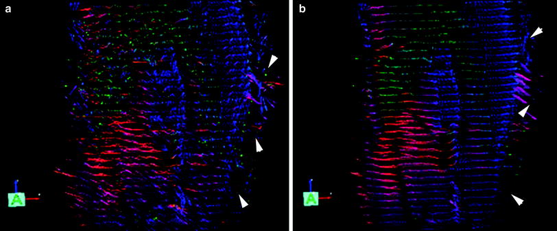
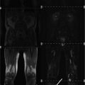
Fig. 4

The leading eigenvector is shown in both images as arrows with the color indicating vector direction with the following color map (blue superior-to-inferior direction, red medial to lateral direction, and green anterior to posterior direction). The left image (a) is unsmoothed and the right image (b) is the corresponding smoothed image. Large eigenvectors outside the muscle (indicated by white arrowheads) correspond to fat regions and show erroneous fractional anisotropy and eigenvector directions [Reprinted with permission from Sinha et al. (2011)]

5.2 Geometric Distortions from Eddy Currents and Motion

The diffusion-weighted images have geometric distortions from eddy currents arising from the large diffusion gradients (Sinha et al. 2011; Sinha and Sinha 2011; Heemskerk et al. 2010; Froeling et al. 2012). This distortion and motion correction is performed by an affine transform to the baseline image volume of the diffusion-weighted data. The affine transformation is used to reorient the b-matrix as well (Leemans and Jones 2009).

5.3 Geometric Distortions from Susceptibility Artifacts

This artifact arises from magnetic field inhomogeneities primarily due to susceptibility differences in adjacent structures. The field inhomogeneities result in a spatial mis-mapping with regions of signal loss and signal pile-up. The extent of distortions is the same in the baseline and in the diffusion-weighted images. Most muscle DTI studies do not correct for this artifact. However, it is important to correct for these geometric distortions in order to perform accurate fiber tractography, correlate morphological to diffusion tensor data, and to enable image-based modeling. Methods used in brain diffusion tensor imaging have been extended to muscle diffusion data. One method that has been implemented is based on acquisition of phase images which map the field inhomogeneity; these phase values can be used to directly assign voxels to the correct location (Froeling 2012; Froeling et al. 2012). This approach, however, requires an additional double echo gradient echo scan and it is not clear if it will work when parallel imaging is used. An alternate approach is to nonlinearly deform the baseline image of the diffusion-weighted dataset to a geometrically accurate structural image and apply the deformation to the diffusion tensor calculated from the uncorrected data (Sinha et al. 2011; Sinha and Sinha 2011). Figure 5 shows the axial slice of the lower leg from the baseline diffusion-weighted image as acquired and the same image after correction with a nonlinear deformation algorithm. The nonlinear deformation was applied to the diffusion tensor rather than to the diffusion-weighted images so that appropriate tensor reorientation can also be performed. The better geometrical match of the corrected data to the structural images can be readily appreciated by the better match of the contours.

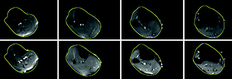
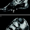
Fig. 5

Top row Corrected baseline images after nonlinear deformation to an image volume acquired using a gradient echo sequence with fat saturation. Bottom row Original baseline images of the diffusion-weighted series. The yellow contour superposed on both image volumes was obtained from the corresponding slice in the gradient echo image. The improvement in geometric fidelity is clearly apparent by a comparison of the contour matching for the two sets

6 Muscle Model of Diffusion

Tseng et al. analyzed diffusion tensor data in myocardial muscle and concluded that the eigenvectors corresponding to the leading, second, and third eigenvalues correspond to the directions along the long axis of the fibers, parallel to the myocardial sheets, and normal to the sheets (Tseng et al. 2003). This myocardial muscle model has been confirmed by histological examination as well (Scollan et al. 1998). Damon et al. were the first to confirm that the pennation angle of the lateral gastrocs fibers in a rat model estimated from DTI is close to that measured by direct anatomical inspection, DAI (Damon et al. 2002). However, the anatomical correlates of the second and third eigenvector of muscle fibers have not yet been conclusively established.

Galbán et al. were the first to suggest a model to explain the observed diffusion tensor eigenvalues in skeletal muscle (Galbán et al. 2004). They proposed that since the lead eigenvector was along the long axis, the second and third eigenvectors are in a plane orthogonal to the long axis. The second eigenvector is hypothesized to run along the sheets of individual muscle fibers within the endomysium, the region between the fibers. The eigenvector associated with the third eigenvalue is then related to transport pathways with the muscle in this model. They verified the model prediction that PCSA is proportional to the third eigenvalue in the lower leg muscles.

An extension of this model was advanced to account for gender-based differences in DTI indices: the extended model includes the muscle fiber volume fraction in a well-defined arbitrary muscle volume (Galbán et al. 2005). The extended model predicts that a larger volume fraction of skeletal muscle in males is muscle fibers (anisotropic hindered diffusion) compared to females who have a larger fraction of endomysium (isotropic, less hindered diffusion); this was verified in their study as females had a larger ADC values while males had higher FA values (Galbán et al. 2005).

Karampinos et al. proposed an interesting diffusion tensor model which took into account the cross-sectional asymmetry of muscle fiber geometry (Karampinos et al. 2007, 2009). In their model, diffusion occurs in a space composed of the space within the muscle fiber and the extracellular space. The muscle fibers themselves were modeled as cylinders of infinite length with an elliptical cross-section with dimensions derived from histological studies of excised muscle. In the model, λ ₂ and λ ₃ (the second and third eigenvalues) reflect the principal diameters of the elliptical cross-sectional area of the myofibrils. Though there is no complete validation as yet for the second and third eigenvector directions, the elliptical cross-sectional model has some support since the second eigenvector has been tracked in a recent study (Gharibans et al. 2011).

It is also possible to infer the link between the eigenvalues and the fiber microarchitecture by looking at changes on flexion. Consistent changes have not been reported for plantarflexion, but most studies show that λ ₃ increases. This is in line with the models relating λ ₃ to muscle diameter. In the elliptical cross-sectional model, if there is isotropic deformation in the fiber cross-section, similar increases in λ ₂ should be expected. However, evidence from other studies such as strain rate tensor (Englund et al. 2011; Sinha et al. 2012), show that fiber cross-sectional deformation is highly anisotropic. This suggests that if deformation is only along one direction, λ ₂ should not change as much as λ ₃. Experimental evidence of small changes in λ ₂ with flexion comes from Hatakenaka et al. (2008) and Sinha et al. (2011). However, other studies have reported both decreases and increases in λ ₂ (Deux et al. 2008). More studies using robust acquisition and post-processing techniques are required to document changes in the diffusion indices with flexion; such studies may help elucidate the diffusion model in the musculoskeletal (MSK) system.

7 Diffusion Tensor Indices in the Normal MSK System

Detailed analysis of the DTI of the forearm muscles have been reported by Froeling et al. (2012). The eigenvalues, MD, and FA were calculated for six muscles of the forearm as well as for the whole muscle volume. Typical values for the MD in the whole muscle of the forearm were 1.49 ± 0.09 × 10⁻⁹ m²/s and FA values were 0.30 ± 0.02. Values reported for the MG of the lower leg are 1.32 ± 0.06 × 10⁻⁹ m²/s and FA values were 0.23 ± 0.04 (Sinha and Sinha 2011). The same group also extracted the diffusion indices for the different compartments of the soleus (Sinha et al. 2011): MD and FA of posterior soleus: 1.47 ± 0.06 × 10⁻⁹ m²/s and 0.20 ± 0.04; MD and FA of anterior soleus: 1.60 ± 0.08 × 10⁻⁹ m²/s and 0.20 ± 0.04. Heemskerk et al. reported the values in anterior tibialis (TA) for the mean diffusivity as 1.64 ± 0.05 × 10⁻⁹ m²/s and for the FA as 0.23 ± 0.04 (Heemskerk et al. 2010). Heemskerk et al. also determined the coefficient of variation (CV) for the diffusion indices, fiber orientation, and lengths. They report CV of <3 % for the eigenvalues and MD, <8 % for the FA, and the repeatability coefficients of the fiber pennation angle and length to be less than 10.2 and 50 mm, respectively. The above measurements of normal diffusion indices in skeletal muscle were performed at 3 T. A comparison of 1.5 and 3 T scanners based on two subjects scanned on 3 days to calculate the coefficient of variability (CV) showed that the values for the DTI indices as well as for the fiber orientation were in a similar range (<3 % for the eigenvalues, <8 % for the FA, and 8–12 % for the fiber orientation). Given the widespread availability of 1.5 Tesla scanners, this opens the possibilities for using DTI to monitor muscle architecture in normal and diseased states (Sinha and Sinha 2011).

The repeatability studies allow one to determine if the measurement precision is sufficient to detect changes with disease state. DTI indices are known to change in the range of 10–20 % in diseased or damaged tissue (Heemskerk et al. 2006, 2007; Qi et al. 2008). The RC of the DTI indices (eigenvalues, FA) in the lower leg muscles is reported to be less than 10 %, and thus the DTI sequences should be capable of detecting changes in muscle DTI indices with disease/damage. Changes in muscle architecture arising from changes in ankle positions or from contraction can be as small as 3–5°, so that repeatability coefficients for fiber orientations should be in this range. The average RCs of the fiber orientations in prior reported studies is ~8°, which is more than the anticipated changes in fiber orientation with ankle position or from contraction. However, it should be noted that muscle architecture changes are typically monitored without any change in patient position, so that these measurements (same session, no subject repositioning) will have a higher reproducibility than that measured on separate days with subject repositioning. This is probably the reason that fiber orientation changes of the order of 8° could be detected even when the RC value was in the same range (Sinha et al. 2011; Sinha and Sinha 2011).

7.1 Diffusion Tensor Imaging Under Passive and Active Muscle Contraction

There have been varying reports on the changes under passive and active muscle contraction. Hatakenaka reported that in the medial gastrocnemius (mGM) passive contraction resulted in a decrease in λ ₁, no change in λ ₂ and an increase in λ ₃ which lead to a lower FA value (Hatakenaka et al. 2008). The opposite effect was seen in the TA. Duex et al. reported that in the mGM, the three eigenvalues and ADC increased while FA decreased during an active contraction from neutral to plantarflexion (Deux et al. 2008). The reverse trend was observed in the TA. Okamoto et al. also performed DTI under active contraction and found higher values for λ ₁ and λ ₂ as well as FA in the mGM with an opposite effect for the TA and attributed some of the changes to changes in focal temperature and perfusion (Okamoto et al. 2010). Schwenzer et al. measured orientation changes in the soleus under neutral and plantarflexed ankle positions (Schwenzer et al. 2009). For the soleus, they report increase in λ ₂ and λ ₃, no change in λ ₁, a decrease in FA, and a small change of 4° in the fiber orientation with respect to the z-axis. Sinha et al. report much larger changes in the soleus when the foot is in the neutral and plantarflexed states (~60° in the posterior soleus) (Sinha et al. 2011).

Hatakenaka have built on diffusive models in skeletal muscle in the literature to propose a model for contraction (Hatakenaka et al. 2008). Sarcomeres (2 μm length) are shortened on contraction, while muscle fiber cross-sectional diameter (40–120 μm), as well as that of myofibrils (3 μm), increase. Since myofibril dimensions are of the order of the observed diffusion lengths (10 μm), the diffusion in the radial direction increases due to increase in myofibril diameter; this is confirmed by observations on λ ₃. Hatakenaka also suggested that sarcomere shortening may contribute to a decrease in λ ₁ (Hatakenaka et al. 2008). Other models propose that λ ₁ should not change with contraction as whole muscle fiber lengths are far greater than diffusion lengths, resulting in λ ₁ being insensitive to muscle fiber length changes (Schwenzer et al. 2009). The increase in λ ₃ seen in several studies can be attributed to an increase in muscle fiber diameter as the muscle contracts on plantarflexion. However, both experimental data and models are not consistent and more studies on flexion may help identify consistent changes in diffusion indices and may ultimately provide clues to the correct diffusion model.

Only gold members can continue reading. Log In or Register to continue