and Mixed Multichannel Denoising Using Statistical Halfspace Depth Functions

which successively shifts through an image I of size $W\times H$ . This can be expressed as follows [13, 15]:

$\begin{aligned} result\_I(x,y)\,=\,\sum _{s\,=\,-\frac{w_{mask} }{2}}^{\frac{w_{mask} }{2}} \;{ \sum _{t\,=\,-\frac{h_{mask} }{2}}^{\frac{h_{mask} }{2}} {M(s,t){*}I(x+s,y+t)} } \end{aligned}$

(1)

Linear spatial domain filters preserve the edges and perform well in removal of monochromatic Gaussian type noises (e.g. white or random), and in edge detection in images corrupted by impulse noise [13, 15]. However, they become less effective for higher noise powers, reduce edge sharpness, blur the lines and fine details on an image, and are not efficient in removing the signal-dependent noise [13, 15]. This led to development of improved linear spatial domain filters like Wiener filters, although Wiener filters require both noise and signal spectrum information, and can be applied only to smooth underlying signals [13].

Nonlinear spatial domain filters overcome many of the linear filters’ drawbacks, and have proven their competence in elimination of impulse, uniform and fixed valued noises, without need for their explicit identification [13]. Baseline median filter implements the filtering technique expressed by Eq. (1), and is still very broadly used due to its speed and tendency to preserve the edges under certain conditions [13]. Primarily, it is applied in removal of monochromatic impulse noise with fixed noise power values (e.g. salt-and-pepper). As Eq. (1) shows, median filter like many other spatial domain filters, affects every pixel in an image, both those corrupted and uncorrupted by noise; hence, the resulting images are often blurred and have untraceable edges [13]. Many improved nonlinear spatial domain filters have been proposed in order to improve these shortcomings [13, 41]. Such filters are, for example, centre weighted median (CWM) and switching median (SM) filters which are widely implemented in removal of monochromatic impulse noise with fixed values [5, 13], and filters like adaptive CWM, adaptive SM, and progressive switching median which have been introduced for removal of random-valued monochromatic impulse noise [5, 9].

With increasing need for multichannel denoising, numerous spatial domain nonlinear filters have been proposed mostly for elimination of multichannel impulse noise [5, 26]. Early stage filters like marginal (component-wise) median filter (MMF) often applied the method of scalar filtering of each channel individually [4, 5, 16, 26]. In this way, the inherent spectral correlation between channels is ignored which commonly causes the appearance of colour artefacts in resulting images. To date, this issue has been mainly resolved using numerous vector filtering techniques which essentially consider multichannel images as vector fields, and process multichannel pixels as vectors. They have been very successfully applied in elimination of multichannel impulse noise, and can be classified into eight categories [5]:

basic vector filters
adaptive fuzzy vector filters
hybrid vector filters
adaptive centre-weighted vector filters
entropy vector filters
peer group vector filters
vector sigma filters
miscellaneous (other) vector filters

However, basic, adaptive fuzzy, and hybrid vector filters are applied to all pixels in an image, even those not corrupted by noise; this may lead to disappearance of fine image details, blurred edges and overall excessive smoothness of resulting images [5, 13]. As a response to these issues, intelligent filters have been proposed which attempt to discern the pixels corrupted by noise from those that are not [4, 5]. Once the noisy pixels are identified, some of the vector filters (e.g. based on robust order statistics) are used; in other words, these filters switch between the identity operation and a vector filtering method, depending on some predetermined criteria. Consequently, they have reduced computational costs since a time-consuming filtering process is only executed on selected pixels observed as noisy [4, 5].

In contrast to the advancement of multichannel impulse and additive denoising filters, only a small number of filtering methods (both spatial and transform domain) have been suggested so far for removal of mixed multichannel noise [9, 50, 62].

A completely novel concept of multichannel filtering based on statistical depth functions, or more precisely, statistical halfspace depth function is discussed in this chapter. Resulting halfspace deepest location filter (HSDLF) offers outstanding results in elimination of impulse and mixed multichannel noise [2, 3]. Even though HSDLF belongs to the class of spatial domain filters, its underlying algorithm is substantially different to nonlinear vector (as well as other) impulse noise filters, and transform domain filters. HSDLF filtering method is based on an adjusted version of the DEEPLOC algorithm [60] which calculates the approximate value of multivariate median (i.e. deepest location or the most central point within a data cloud) in d-dimensional space. Its multivariate/multidimensional character ensures that HSDLF intrinsically considers all channels in a multichannel image simultaneously, thus preserving the spectral correlation between channels.

HSDLF does not depend on the source and/or distribution of multichannel noise, and its efficiency in removal of:

multichannel (colour) impulse noise in both of its common variations: salt-and-pepper noise (with fixed values of pixel noise) and random-valued multichannel noise (with arbitrary values of pixel noise) [2], and
multichannel (colour) mixed noise, i.e. mixture of impulse (precisely, salt-and-pepper) and additive Gaussian multichannel noise (ACGN) [3],

has been verified.

Denoising results of HSDLF are compared in terms of objective error metrics (effectiveness) criteria and visual quality to:

marginal median multichannel filter (MMF) [16] and 25 most significant state-of-the-art multichannel impulse noise filters [1, 4, 6–8, 16–24, 27–38, 40, 43–45, 54–59, 61] for impulse multichannel noise removal
two state-of-the-art DWT based filters for removing multichannel Gaussian type noise: Probshrink [42] and BM3D (image denoising by sparse 3D transform-domain collaborative filtering) [11], as well as 26 filters for removal of multichannel impulse noise [1, 4, 6–8, 16–24, 27–38, 40, 43–45, 54–59, 61] for mixed multichannel noise removal

2 Halfspace Depth Function and Computation of Deepest Location for Multivariate Data

Finding the centre set of points within a multidimensional data cloud and generalisation of notion of median in multivariate case have been widely discussed in the literature [10, 12, 25, 39, 47–49, 53, 60, 63–65]. Since these notions cannot be directly derived from their univariate equivalents, several approaches have been introduced to address these issues with theory of statistical depth functions being the most prolific of them all. With their emerging popularity, many statistical depth functions have been formulated; Zuo and Serfling made a thorough overview and classification of all significant statistical depth functions [65]. HSDLF applies the most important representative entitled halfspace (Tukey’s or location) depth function [25, 60, 63, 65].

2.1 Definition and Properties of Halfspace Depth Function

Associated with a given probability distribution P on d-dimensional real space $\mathbb {R}^{d}$ , statistical depth functions provide a P-based centre-outward ordering (and thus ranking) of points (or more precisely, Borel sets) $\varvec{\theta } \in \mathbb {R}^{d}$ . The essential example of statistical depth functions is the halfspace (Tukey’s or location) depth function $HD\left( {\varvec{\theta } ;P} \right)$ which can be defined through following equation [25, 60, 65]:

$\begin{aligned} HD\left( {\varvec{\theta } ;P} \right) \hbox {=}\inf \left\{ {P\left( H \right) :\varvec{\theta } \in H\,\text {closed halfspace}} \right\} ,\;\varvec{\theta } \in \mathbb {R}^{d} \end{aligned}$

(2)

In other words, halfspace depth (HD) function denotes the minimal probability attached to any closed halfspace with ${\varvec{\theta }}$ on the boundary. In a discrete case, the halfspace depth function $HD\left( {\varvec{\theta } ;{\varvec{X}}_n } \right)$ of a point $\varvec{\theta } \in \mathbb {R}^{d}$ relative to a data set ${\varvec{X}}_n \,=\,\left\{ {{\varvec{x}}_1 ,{\varvec{x}}_2 \ldots {\varvec{x}}_n } \right\} \in \mathbb {R}^{d\times n}$ represents the smallest number of observations (elements of ${\varvec{X}}_n \in \mathbb {R}^{d\times n})$ in any closed halfspace with boundary through point ${\varvec{\theta }}$ [63]. Multivariate halfspace depth can be also expressed using its univariate case $HD_1 \left( {\theta ;{\varvec{X}}_n } \right)$ [60]:

$\begin{aligned} HD_1\left( {\theta ;{\varvec{X}}_n } \right) \,=\,HD\left( {\varvec{\theta } ;{\varvec{X}}_n } \right) \mid {_{d\,=\,1} } \,=\,\min \left( {\# \left\{ {x_i \le \theta } \right\} ,\# \left\{ {x_i \ge \theta } \right\} } \right) \end{aligned}$

(3)

where # is a number of observations.

This definition interprets the halfspace depth $HD\left( {\varvec{\theta } ;{\varvec{X}}_n } \right)$ as the smallest univariate halfspace depth value of a point ${\varvec{\theta }}$ relative to any projection of the data set ${\varvec{X}}_{ {n}}$ onto a direction ${\varvec{u}}$ [60]:

$\begin{aligned} \begin{array}{l} HD(\varvec{\theta } ;{\varvec{X}}_n )\,=\,\mathop {\min }\limits _{\left\| u \right\| \,=\,1} \;HD_1 \left( {\varvec{u}}'\varvec{\theta } ;{\varvec{u}}'{\varvec{X}}_n \right) \,=\,\mathop {\min }\limits _{\left\| u \right\| \,=\,1} \left( {\min \left( {\# \left\{ {{\varvec{u}}'{\varvec{x}}_i \le {\varvec{u}}'\varvec{\theta } } \right\} ,\# \left\{ {{\varvec{u}}'{\varvec{x}}_i \ge {{\varvec{u}}}'\varvec{\theta } } \right\} } \right) } \right) \\ \quad \quad \quad \quad \; =\mathop {\min }\limits _{\left\| u \right\| \,=\,1} \;\# \left( {i;{\varvec{u}}'{\varvec{x}}_i \le {\varvec{u}}'\varvec{\theta } } \right) \end{array} \end{aligned}$

(4)

It means that halfspace depth $HD\left( {\varvec{\theta } ;{\varvec{X}}_n } \right)$ indicates how deep a point $\varvec{\theta }$ is centred within the data cloud (set). Additionally, halfspace depth is defined as multivariate ranking: points nearer the boundary of the data set have lower ranks, and the rank increases as one gets deeper inside the data cloud [60]. Ranking can be geometrically illustrated using the notion of halfspace depth regions ${ D}_{l}$ defined by equation:

$\begin{aligned} D_l \,=\,\left\{ {\varvec{\theta } \in \mathbb {R}^{d};\;H D(\varvec{\theta } ;{\varvec{X}}_n )\ge l} \right\} \end{aligned}$

(5)

Halfspace depth regions are convex sets, and for every HD and l, $D_l \subseteq D_{l-1}$ holds [60]. Boundary of a region with equivalent HD values is called halfspace depth contour. Unique centre of gravity of the smallest halfspace depth region $D_{l_{max} }$ which contains the points with maximal HD values (equal to $l_{max}$ ) can be interpreted as multivariate median, i.e. a generalisation of univariate median to multidimensional spaces [60]. It also called Tukey’s median or the deepest location.

Zuo and Serfling have shown that halfspace depth function $HD\left( {\varvec{\theta }} ;P \right)$ fulfils all useful and desirable properties required of a statistical depth function [65]:

Affine invariance. $HD\left( {\varvec{\theta }} ;P \right)$ is independent of the coordinate system.
Maximality at center. If P is symmetric about ${\varvec{\theta }}$ in some sense, then $HD\left( {\varvec{\theta }} ;P \right)$ is maximal at this point.
Symmetry. If P is symmetric about $\varvec{\theta }$ in some sense, then so is $HD\left( {\varvec{\theta }} ;P \right)$ .
Decreasing along rays. The depth $HD\left( {\varvec{\theta }} ;P \right)$ decreases along every ray from the deepest point.
Vanishing at infinity. $HD\left( {\varvec{\theta }} ;P \right) \rightarrow 0,\;\left\| {\varvec{\theta }} \right\| \rightarrow \infty$ .
Continuity of $HD\left( {\varvec{\theta }} ;P \right)$ as a function of ${\varvec{\theta }}$ (upper semicontinuity).
Continuity as of $HD\left( {\varvec{\theta }} ;P \right)$ a functional of P.
Quasi-concavity as a function of ${\varvec{\theta }}$ . The set $\left\{ {\varvec{\theta }} :HD\left( {\varvec{\theta }} ;P \right) \ge c \right\}$ is convex for each real c.

Affine invariance is a particularly useful property for calculation of deepest location; in case of HD, this means that for any affine transformation $g:\mathbb {R}^{d}\rightarrow \mathbb {R}^{d}:{\varvec{x}}\rightarrow A\cdot {\varvec{x}}+{\varvec{b}}$ , with ${\varvec{b}}\in \mathbb {R}^{d}$ and $A\in \mathbb {R}^{d\times d}$ a nonsingular matrix, equality $HD\left( {g(\varvec{\theta } );g({\varvec{X}}_n )} \right) \,=\,HD\left( {\varvec{\theta } ;{\varvec{X}}_n } \right)$ holds. Consequently, the deepest location (Tukey’s median) ${\varvec{M}}_{DL}^{HD}$ is also affine equivariant: ${\varvec{M}}_{DL}^{HD} \left( {g({\varvec{X}}_n )} \right) \,=\,g\left( {{\varvec{M}}_{DL}^{HD} ({\varvec{X}}_n )} \right)$ .

Furthermore, Tukey’s median is a very robust multivariate location estimator, and its robustness can be evaluated by means of the breakdown value $\varepsilon ^{*}$ . As proven by Donoho and Gasko [12], Tukey’s median ${\varvec{M}}_{DL}^{HD}$ satisfies the inequality $\varepsilon ^{*}\left( {{\varvec{M}}_{DL}^{HD} ;{\varvec{X}}_n } \right) \ge \frac{n}{d+1}$ for any sample in general position. This means that the resulting Tukey’s median ${\varvec{M}}_{DL}^{HD}$ will not move outside of a bounded region if $\frac{n}{d+1}$ observations are replaced from the data set ${\varvec{X}}_{n}$ . If the original data set ${\varvec{X}}_{n}$ comes from any angularly symmetric distribution, and especially from an elliptically symmetric distribution, the breakdown value $\varepsilon ^{*}\left( {\varvec{M}}_{DL}^{HD} ;X_n \right)$ tends to $\frac{1}{3}$ in any dimension. Simply put, if at least 67 % of the data points in ${\varvec{X}}_{n}$ are drawn from such a distribution then the deepest location remains within reasonable limits, regardless of the other points in the data set.

In general, not many algorithms have been proposed for calculation of statistical depth functions. A number of algorithms for computation of halfspace depth have been proposed in the literature [10, 47–49, 60, 64]; however, only a few algorithms for finding multivariate halfspace deepest location (Tukey’s median) have been proposed: [48] for bivariate data, and, [10, 47] and [60] for dimensions more than two. DEEPLOC algorithm [60] has been selected as a basis of HSDLF, primarily because it implements the only mathematically proven and exact algorithm for calculation of halfspace depth functions in $\mathbb {R}^{3}$ [49, 60]. Most importantly, it has been shown that approximate location depth calculated with DEEPLOC is very close to the exact depth for real data sets [60].

2.2 Finding the Deepest Location Using DEEPLOC Algorithm

DEEPLOC algorithm computes an approximation of deepest location (Tukey’s median) for any dimension d. It works with a subset of directions u [see Eq. (4)] to approximate the halfspace depth, and is constructed to be the least time consuming [49, 60]. DEEPLOC algorithm and its stepwise pseudocode are presented in their full (and complex) details in the original work of Struyf and Rousseeuw [60]. In this section only the most significant steps in DEEPLOC are explained which are of importance for understanding of how HSDLF works. Also, the places where the original DEEPLOC algorithm is altered are indicated.

In short, DEEPLOC starts from an initial point and takes further steps in carefully selected directions in which the halfspace depth can be increased (unlike the solution proposed in [10]), so that the deepest location (Tukey’s median) can be approached after several of these steps. In order to reduce the number of steps, a centrally located initial point like coordinate-wise median or (affine invariant) coordinate-wise mean is taken, since it gives a fairly good halfspace depth relative to the data set, and is easy to compute [60]:

$\begin{aligned} {\varvec{M}}_1 \,=\,\left( {Med (x_{i1} ;i\,=\,1,\ldots n),\ldots ,Med(x_{id} ;i\,=\,1,\ldots n)} \right) \end{aligned}$

(6)

After calculating the starting point, m directions ${\varvec{u}}\in \mathbb {R}^{d}$ are constructed with $\left\| {\varvec{u}} \right\| \,=\,1$ . These directions are randomly drawn from following classes [60]:

(a)

d coordinate axes

(b)

vectors connecting an observation with ${\varvec{M}}_{1}$

(c)

vectors connecting two observations

(d)

vectors perpendicular to a d-subset of observations

Classes (a), (b) and (c) are included as they are easy to compute, and are used for detection of marginal and far outliers [60]. However, class (d) directions are of greatest importance due to their close relation to halfspace depth notion, thus the majority of directions are taken from it. As a basis, HSDLF uses the proportion of directions from the original DEEPLOC algorithm [60]:

all directions from the class (a)
at most m/4 directions from each of the classes (b) and (c)
at least m/2 directions from the class (d)

However, an additional parameter which controls the distribution of directions is introduced in HSDLF, and is called threshold control parameter (see Sect. 3). The overall number of directions m can be given by the user and in case of HSDLF, m = 500 directions are computed by default (see Sect. 3).

Univariate halfspace depth of ${\varvec{M}}_{1}$ relative to the projection of ${\varvec{X}}_{n}$ on each of these m directions is then computed. The directions u which lead to the same lowest value $\# \left\{ {i;{\varvec{u}}'{\varvec{x}}_i \le {\varvec{u}}'{\varvec{M}}_1} \right\}$ are stored in set ${ U}_{move}$ , and these directions are considered as the ones in which the halfspace depth is able to improve [60]. The average direction ${\varvec{u}}_{move}$ of directions saved in set ${ U}_{move}$ is then calculated:

$\begin{aligned} {\varvec{u}}_{move} \,=\,\frac{1}{\left| {U_{move} } \right| }\sum _{{\varvec{u}}\in U_{move}} {\varvec{u}} ,\text {where} \quad {\varvec{u}}_{move} \ne \mathbf{0} \end{aligned}$

(7)

After that, a step is taken from ${\varvec{M}}_{1}$ in the direction of ${\varvec{u}}_{move}$ . As mentioned, the value of halfspace depth at the deepest location relative to ${\varvec{X}}_{n}$ has to be at least $\left[ {\frac{n}{d+1}} \right]$ (where square brackets represent the floor function). If this condition is not fulfilled for ${\varvec{M}}_{1}$ , i.e. if following inequality holds:

$\begin{aligned} H D_1 \left( {{\varvec{M}}_1 ;{\varvec{u}}'_{move} {\varvec{X}}_n} \right) <\left[ {\frac{n}{d+1}} \right] \end{aligned}$

(8)

a step in the direction ${\varvec{u}}_{move}$ is taken, which is large enough to reach a point ${\varvec{M}}_{2}$ which has univariate halfspace depth value of $\left[ {\frac{n}{d+1}} \right]$ . Otherwise, a step is taken in the direction ${\varvec{u}}_{move}$ to the point ${\varvec{M}}_{2}$ which has univariate halfspace depth larger for 1 unit than the halfspace depth of ${\varvec{M}}_{1}$ in the same direction ${\varvec{u}}_{move}$ [60].

Afterwards, the explained procedure is repeated with ${\varvec{M}}_{2}$ (or ${\varvec{M}}_{next}$ in iteration for next $$$>$$” src=”/wp-content/uploads/2016/03/A308467_1_En_5_Chapter_IEq76.gif”>2) taking the roll of the initial point (<IMG alt=$${\varvec{M}}_{1}$$ src=$ in previously described algorithm steps) until a point ${\varvec{M}}_{maxHD}$ is found with maximal halfspace depth of $\frac{n}{2}$ , or until the algorithm stops showing any halfspace depth improvement in previous ${ N}_{try}$ iteration steps. If the algorithm begins to oscillate instead of moving towards the deepest location, supplemental features are proposed for reduction of computational cost: if no halfspace depth improvement has been made after ${ N}_{alt}$ successive steps, then the directions connecting some previous points ${\varvec{M}}_{i}$ to the current point $$${\varvec{M}}_{j>i}$$” src=”/wp-content/uploads/2016/03/A308467_1_En_5_Chapter_IEq83.gif”> are considered [<CITE><A href=$ 60]. It should be noted that parameters ${ N}_{try}$ and ${ N}_{alt}$ are also user defined.

Fig. 1

Flowchart illustrating the most significant steps of the DEEPLOC algorithm

Flowchart presented in Fig. 1 illustrates all relevant steps of the DEEPLOC algorithm. Detailed mathematical theorems and their proofs related to the DEEPLOC algorithm are given in [48, 49, 60].

3 Halfspace Deepest Location Filter

DEEPLOC pseudocode served as a foundation of the HSDLF’s programming code [2, 3]. During the experiments (see Sect. 4), it has been empirically established that a slight increase in number of directions from class (d) (defined in Sect. 2.2) improves filtering results. In order to give HSDLF an additional degree of freedom and even more flexibility, a scalar parameter entitled threshold control parameter $\tau$ was introduced with values ranging from 0 to 1, which controls the percentage of class (d) directions¹. As directions from class (d) play the vital role in DEEPLOC algorithm, parameter $\tau$ aims to provide fine-tuning of HSDLF’s output results and precision. Experiments have shown that this small increase in number of class (d) directions has an insignificant impact on computational cost [2, 3].

HSDLF applies this adjusted version of the DEEPLOC algorithm for calculating deepest location (Tukey’s median) in three dimensional space (d = 3 in notation of Sects. 2.1 and 2.2), where R, G and B colour channels act as dimensions (coordinates). It was assumed that the multichannel images are 24-bit (8-bit per channel), so the values of R, G and B channels range from 0 to 255 for each channel.

HSDLF uses the standard spatial filtering technique based on a sliding convolution kernel (filtering window) described in Sect. 2 [2, 3]. Let ${ r}_{ij}$ , ${ g}_{ij}$ , and ${ b}_{ij}$ denote the values of red, green, and blue channels, respectively, of a pixel at the position (i,j) in an image I of size $W\times H$ contaminated by multichannel noise, i.e. $I\,=\,\left\{ {(r_{ij} ,g_{ij} ,b_{ij} )|1\le i\le W,1\le j\le H} \right\}$ . Convolution kernel M of size $k\times k$ , where k is an odd positive integer, includes the pixel positioned at the centre of kernel M, i.e. (i,j) in the image I, and $k^{2}-1$ of its neighbouring pixels. This means that the kernel M enfolds $k^{2}$ ordered triplets of red, green and blue channel values, respectively, of corresponding pixels. HSDLF computes the deepest location within a data cloud which consists of these $k^{2}$ three dimensional data using the adjusted DEEPLOC algorithm, and replaces the channel values of pixel at the centre of kernel M ((i,j) in image I) with estimated deepest location’s channel values. Image edges are handled identically as in standard (marginal) median filters.

Number of directions is kept at a fixed value of m = 500 since this is the minimum value of m for which HSDLF gives excellent balance between high performance and computation time. It was shown that the algorithm accuracy gradually increases with an increase in number of directions m; however, the computational cost grows rapidly [2, 3].

In early stages of HSDLF testing on 24-bit multichannel images, it was noted that deepest location channel values in very rare cases with far outliers can be negative (precisely, take value

), or can exceed the limit of 255 (precisely, take value of 256). In order to preserve the visual smoothness and consistency of filtered images without affecting the computational cost, these particular pixels are additionally filtered with MMF [5], which is very fast and calculated analogously to HSDLF. This correction would not be needed if the number of directions m was set to value of more than 1,500 or if another colour system such as CIELab or YCbCr was used. However, in the latter case, a different range of channel values in these colour systems sometimes causes difficulties in calculation of location depth/deepest location.

Fig. 2

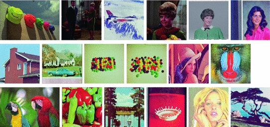
Benchmark images used for comparison of all observed filters’ denoising performances, from left to right (image dimensions in pixels are given in brackets): Caps (768 $\,\times \,$ 512), Couple (256 $\,\times \,$ 256), F16 (512 $\,\times \,$ 512), Girl1 (256 $\,\times \,$ 256), Girl2 (256 $\,\times \,$ 256), Girl3 (256 $\,\times \,$ 256), House (256 $\,\times \,$ 256), House With Car (512 $\,\times \,$ 512), Jellybeans1 (256 $\,\times \,$ 256), Jellybeans2 (256 $\,\times \,$ 256), Lena (512 $\,\times \,$ 512), Mandrill (512 $\,\times \,$ 512), Parrots (768 $\,\times \,$ 512), Peppers (512 $\,\times \,$ 512), Sailboat (512 $\,\times \,$ 512), Splash (512 $\,\times \,$ 512), Tiffany (512 $\,\times \,$ 512), and Tree (256 $\,\times \,$ 256)

It is important to point out that in case of the image set used in Sect. 4 for all observed types and/or powers of multichannel noise, and observed values of threshold control parameter $\tau$ , the filtering results with and without this MMF correction are identical, and no cases of deepest location values going out of $\left[ {0,255} \right]$ range appear on this image data set, even though the number of directions m is set to 500 [2, 3]. Also, HSDLF evidently does not depend on the nature or powers of applied multichannel noise; therefore, it can be used for elimination of many types of multichannel noise regardless of their origin [2, 3].

4 Experimental Results and Their Analysis

Performance of HSDLF has been tested on some of the most commonly used 24-bit multichannel (8-bit per colour channel) benchmark images: Signal and Image Processing Institute (SIPI) Volume 3: Miscellaneous image database set, with addition of two more images (“Parrots” and “Caps”) from the Kodak Photo CD PCD0992 [2, 3]. These 24-bit (i.e. 8-bit-per-channel) multichannel benchmark images have fixed image sizes of $256\,\times \,256$ pixels (“Couple”, “Girl1”, “Girl2”, “Girl3”, “House”, “Jellybeans1”, “Jellybeans2”, “Tree”), $512\,\times \,512$ pixels (“F16”, “House With Car”, “Lena”, “Mandrill”, “Peppers”, “Sailboat”, “Splash”, “Tiffany”) and $768\,\times \,512$ pixels (“Caps”, “Parrots”) (see Fig. 2).

However, due to very large amount of data, comparison of HSDLF’s performance against 28 state-of-the-art filters will be presented for four essential benchmark images, namely “Lena” and “Peppers” (with sizes of 512 $\,\times \,$ 512 pixels) from Signal and Image Processing Institute (SIPI) Volume 3: Miscellaneous image database, and “Parrots” and “Caps” (with sizes of 768 $\,\times \,$ 512 pixels) from Kodak Photo CD PCD0992.

In all experiments, the convolution kernel (sliding filtering window) size is set to $3\times 3$ (see Sect. 3). HSDLF results have been produced using Simple DirectMedia Layer and CImg open source libraries within C++ programming language framework. Consequently, HSDLF does not require any specific digital image format, and can be successfully applied to nearly all digital image formats, including lossy compressed formats like JPEG. All types of noise have been generated using MATLAB R2011a software.

4.1 Multichannel Impulse Noise Removal

As mentioned in Sect. 1, performances of HSDLF and other multichannel impulse noise filters are compared on images corrupted by salt-and-pepper as well as random-valued noise, with following power levels/densities applied: $\xi \,=\,\{ 0.1,\;0.2,\;0.3,0.4,\;0.5 \}$ .

Salt-and-pepper noise on image I is generated using MATLAB built-in $imnoise\left( {I, 'salt\hbox { } \& \hbox { }pepper',\xi } \right)$ function where $\xi$ denotes the noise density. This means that approximately $\xi \cdot \hbox {number}\;\hbox {of}\;\hbox {pixels}(I)$ randomly chosen pixels are replaced by pixels which have values of 0 or 255 on each channel (red, green and blue). Random-valued noise with density $\xi$ on image I is generated indirectly since MATLAB does not have a built-in function for its production. Using the built-in MATLAB function $$rand$$

for generation of uniformly distributed pseudorandom numbers, $\xi \cdot \text {number}\;\hbox {of}\;\hbox {pixels}(I)$ pixels are selected randomly and then replaced by pixels with random values ranging from 0 to 255 on each colour channel (red, green and blue). Obviously, salt-and-pepper noise could be produced similarly using MATLAB function $$rand$$

; experiments have shown that both of these methods for generating salt-and-pepper noise give identical results [2]. Salt-and-pepper and random-valued noise can be considered as instances of uncorrelated impulsive noise model [5]:

$\begin{aligned} \begin{array}{l} c_{ij}^{(ch)} \,=\,\left\{ {{\begin{array}{l} {r_{ij}^{(ch)} \;\text {with probability }\xi } \\ {o_{ij}^{(ch)} \;\text {with probability 1-}\xi } \\ \end{array} }} \right. \\ \\ r_{ij}^{(ch)} \in \left\{ {{ \begin{array}{l} {\left\{ {0,255} \right\} \;\text {for salt-and-pepper noise}} \\ {\left[ {0,255} \right] \;\text {for random-valued noise}} \\ \end{array} }} \right. \\ \end{array} \end{aligned}$

(9)

where $c_{ij}^{(ch)}$ represents the pixel channel value (red, green or blue) of the output image corrupted by noise, $o_{ij}^{(ch)}$ represents the pixel channel value (red, green or blue) of the original image uncorrupted by noise, and $r_{ij}^{(ch)}$ represents the pixel channel value (red, green or blue) of salt-and-pepper or random-valued noise; ch denotes the colour channel index: ch = 1 for red, ch = 2 green, and ch = 3 blue channel, and $\xi$ symbolises the density of impulse noise that is applied to an image.

HSDLF performance in removal of multichannel impulse noise is compared to marginal median filter MMF [4] and following 25 state-of-the-art impulse noise filters [2, 5]:

adaptive basic vector directional filter ABVDF [29]
adaptive centre-weighted vector filters: ACWDDF [30], ACWVDF [38], ACWVMF [27]
adaptive multichannel nonparametric filter with multivariate exponential kernel function AMNFE [43]
adaptive vector sigma filters: ASBVDF [31–34, 37], ASDDF [31–34, 37], ASVMF [31–34, 37]
adaptive vector median filter AVMF [28]
basic vector directional filter BVDF [61]
directional distance filter DDF [16, 17]
entropy vector filters: EBVDF [35, 36], EDDF [35, 36], EVMF [35, 36]
fast peer group filter FPGF [54]
fuzzy vector median filter FVMF [8, 44, 45]
fuzzy vector median-rational hybrid filter FVMRHF [21–23]
kernel vector median filter KVMF [55–59]
peer group filter PGF [18]
order-statistics based switching vector filters: RSBVDF [7], RSDDF [7]
robust switching vector median filter RSVMF [4]
vector median filter VMF [1]
vector median-rational hybrid filter VMRHF [19, 20, 24]
vector signal-dependent rank order mean filter VSDROMF [40]

Filtering results are compared objectively by means of three error metrics criteria [5]:

peak signal-to-noise ratio (PSNR) in decibels (dB) which measures the noise suppression capability of a filter:

$\begin{aligned} PSNR\,=\,10\cdot \log _{10} \frac{255^{2}}{MSE},\quad MSE\,=\,\frac{1}{3\cdot W\cdot H}\sum _{ch\,=\,1}^3 {\sum _{i\,=\,1}^W {\sum _{j\,=\,1}^H {(\hat{{c}}_{ij}^{(ch)} -c_{ij}^{(ch)} )^{2}} } } \end{aligned}$

(10)
mean absolute error (MAE) which measures the detail preservation capability of a filter:

$\begin{aligned} MAE\,=\,\frac{1}{3\cdot W\cdot H}\cdot \sum _{ch\,=\,1}^3 {\sum _{i\,=\,1}^W {\sum _{j\,=\,1}^H {\left| {\hat{{c}}_{ij}^{(ch)} -c_{ij}^{(ch)} } \right| } } } \end{aligned}$

(11)
where in Eqs. (10) and (11), $\hat{{c}}_{ij}^{(ch)}$ and $c_{ij}^{(ch)}$ represent the pixel channel values of denoised and original images, respectively, and ch symbolises the channel index: ch = 1 for red, ch = 2 green, and ch = 3 blue channel
normalized colour difference (NCD) which measures the colour preservation capability of a filter:

$\begin{aligned} NCD\,=\,\frac{\sum _{i\,=\,1}^W {\sum _{j\,=\,1}^H {\sqrt{\left( {\left( {\hat{{L}}_{ij} -L_{ij} } \right) ^{2}+\left( {\hat{{a}}_{ij} -a_{ij} } \right) ^{2}+\left( {\hat{{b}}_{ij} -b_{ij} } \right) ^{2}} \right) }} } }{\sum _{i\,=\,1}^W {\sum _{j\,=\,1}^H {\sqrt{\left( {\left( {\hat{{L}}_{ij} } \right) ^{2}+\left( {\hat{{a}}_{ij} } \right) ^{2}+\left( {\hat{{b}}_{ij} } \right) ^{2}} \right) }} } } \end{aligned}$

(12)
where $\hat{{L}}_{ij}$ and $L_{ij}$ represent lightness values, and $\left( {\hat{{a}}_{ij} ,\hat{{b}}_{ij} } \right)$ and $\left( {a_{ij} ,b_{ij} } \right)$ chrominance values of denoised and original images, respectively, expressed in CIELAB colour space [32]

Experimental results have shown that HSDLF provides optimal results in removal of multichannel impulse noise for two values of threshold control parameter $\tau$ (0.0015 and 0.005) in terms of both objective error metrics criteria and visual quality [2]. Tested on Signal and Image Processing Institute (SIPI) Volume 3: Miscellaneous and Kodak Photo CD PCD0992 image data sets, it has also been verified that HSDLF performances in multichannel impulse denoising deteriorate quickly for $\tau$ $$>$$” src=”/wp-content/uploads/2016/03/A308467_1_En_5_Chapter_IEq144.gif”>0.006, and slightly for <IMG alt=

$$>$$” src=”/wp-content/uploads/2016/03/A308467_1_En_5_Chapter_IEq144.gif”></SPAN>0.006, and slightly for <SPAN id=IEq145 class=InlineEquation><IMG alt=

0.0012.

Comparison of HSDLF performances in terms of used error metrics criteria for both observed values of the threshold control parameter $\tau$ , calculated for all benchmark images is presented in Table 5. A detailed review of HSDLF performances for both observed types of impulse noise is given in Table 6.

Figures 3, 4 and 5 display the average PSNR, MAE and NCD gain values for all observed impulse denoising filters calculated over all benchmark images. Figures 6a–c, 7a–d, 8a–c, and 9a–d illustrate the visual quality of denoising results of all observed filters applied to image “Caps” corrupted by salt-and-pepper and random-valued multichannel noise, respectively.

The best filtering performances in Tables 1–4 are indicated by $\mathbf{boldface }$ font.

By closely observing the results given in Tables 1, 2, 3, 4, 5 and 6 and Figs. 3, 4, 5, 6a–c, 7a–d, 8a–c, and 9a–d, following conclusions can be drawn [2]:

For all salt-and-pepper and random-valued impulse noise densities and calculated over all observed benchmark images, HSDLF performs better in more than 60% of cases for threshold control parameter value of $\tau$ = 0.0015 than for $\tau$ = 0.005 in terms of PSNR and MAE error metrics criteria, while NCD values are very similar for both values of $\tau$ .
HSDLF denoising results are marginally more sensitive to shifts in values of $\tau$ in terms of all error metrics criteria when the filter is applied to images corrupted by random-valued impulse noise.
PSNR, MAE and NCD gains steadily rise with the increase salt-and-pepper and random-valued noise powers for both HSDLF’s values of $\tau$ on all observed images.

Table 1

Performance results of observed multichannel impulse denoising filters applied to image “Caps” (with $768\,\times \,512$ pixel image size) corrupted by various densities of salt-and-pepper and random-valued impulse noise. The best filtering performances are indicated by $\mathbf{boldface }$ font

		Image: $Caps\,768\,\times \,512$
		0.1			0.3			0.5
	Salt-and-pepper	PSNR	MAE	NCD	PSNR	MAE	NCD	PSNR	MAE	NCD
	noise density	[dB]			[dB]			[dB]
Denoising method	None	17.66	21.36	0.392	12.89	42.83	0.708	10.74	57.86	0.907
	ABVDF	18.09	18.23	0.321	12.39	44.38	0.691	9.95	63.48	0.917
	ACWDDF	20.93	14.13	0.3	15.11	32.17	0.621	12.28	47.09	0.840
	ACWVDF	18.33	18.05	0.332	12.7	42.67	0.692	10.25	60.81	0.917
	ACWVMF	21.88	13.15	0.301	16.02	29.39	0.61	13.12	42.96	0.824
	AMNFE	25.9	8.65	0.197	19.41	20.12	0.427	15.97	31.13	0.603
	ASBVDF	18.31	17.66	0.312	12.91	41.93	0.686	10.56	58.69	0.905
	ASDDF	20.72	14.14	0.29	14.26	35.69	0.64	11.52	51.99	0.865
	ASVMF	22.5	12.37	0.282	16.16	29.18	0.594	13.01	43.71	0.816
	AVMF	20.83	15.01	0.319	16.02	29.93	0.609	13.34	42.15	0.813
	BVDF	18.2	17.62	0.279	12.39	44.48	0.668	9.97	63.49	0.902
	DDF	24.43	9.6	0.213	17.27	24.96	0.525	13.75	39.58	0.753
	EBVDF	17.95	18.56	0.332	12.68	42.98	0.701	10.37	59.96	0.921
	EDDF	20.39	14.38	0.3	14.08	35.96	0.65	11.38	52.47	0.876
	EVMF	22.36	12.56	0.29	16.25	28.83	0.599	13.25	42.54	0.819
	FPGF	23.31	11.36	0.263	17.73	24.18	0.528	14.39	37.04	0.745
	FVMF	25.55	8.74	0.2	18.77	21.27	0.471	15.14	33.81	0.681
	FVMRHF	22.95	11.58	0.276	16.49	27.68	0.595	13.4	41.57	0.816
	KVMF	24.59	9.56	0.223	17.91	23.55	0.517	14.42	36.84	0.742
	MMF	25.26	8.98	0.202	19.13	20.77	0.435	15.7	31.83	0.625
	PGF	22.88	11.77	0.275	17.24	25.38	0.548	14.1	38.21	0.76
	RSBVDF	18.38	18.21	0.344	13.06	41.24	0.698	10.71	57.56	0.913
	RSDDF	21.25	13.56	0.3	14.55	34.5	0.648	11.66	51.05	0.874
	RSVMF	21.94	12.87	0.297	15.25	32.09	0.636	12.23	47.93	0.862
	VMF	24.73	9.34	0.211	17.94	23.49	0.516	14.44	36.78	0.742
	VMRHF	22.69	11.93	0.284	16.37	28.13	0.602	13.32	42	0.823
	VSDROMF	24.21	10.14	0.235	17.88	23.7	0.52	14.43	36.83	0.742
	HSDLF $\tau$ =0.005	27.29	7.58	0.157	22.03	14.55	0.297	18.42	23.12	0.438
	HSDLF $\tau$ =0.0015	27.29	7.58	0.157	22.06	14.49	0.296	18.46	22.99	0.437
		Image: $Caps\,768\,\times \,512$
		0.1			0.3			0.5
	Random-valued	PSNR	MAE	NCD	PSNR	MAE	NCD	PSNR	MAE	NCD
	noise density	[dB]			[dB]			[dB]
Denoising method	None	21.19	13.39	0.252	16.19	27.83	0.477	13.71	39.24	0.637
	ABVDF	21.6	11.72	0.211	15.83	28.53	0.463	13.12	42.11	0.636
	ACWDDF	23.56	9.99	0.203	17.82	22.93	0.431	14.83	34.27	0.597
	ACWVDF	21.71	11.71	0.217	16.04	27.84	0.464	13.31	41.03	0.636
	ACWVMF	24.7	9.07	0.201	18.95	20.38	0.419	15.84	30.58	0.579
	AMNFE	28.62	6.07	0.128	22.02	14.38	0.291	18.06	23.94	0.432
	ASBVDF	22.04	10.76	0.19	16.23	27.19	0.451	13.56	39.81	0.624
	ASDDF	24.53	8.81	0.182	17.72	22.98	0.421	14.52	35.39	0.595
	ASVMF	25.77	8.12	0.183	19.51	19.15	0.398	16.09	29.69	0.562
	AVMF	23.22	10.69	0.217	18.34	22.29	0.435	15.6	31.81	0.589
	BVDF	22.03	10.98	0.17	15.66	29.34	0.432	12.84	44.21	0.615
	DDF	27.42	6.6	0.136	20.46	16.88	0.347	16.67	27.7	0.513
	EBVDF	21.49	11.63	0.207	15.93	28.18	0.465	13.32	41.04	0.637
	EDDF	24.28	8.9	0.187	17.57	23.15	0.429	14.41	35.77	0.605
	EVMF	25.54	8.31	0.189	19.5	19.14	0.402	16.16	29.47	0.565
	FPGF	25.46	8.5	0.19	20.34	17.53	0.373	16.98	26.84	0.522
	FVMF	28.45	6.01	0.128	21.74	14.57	0.311	17.73	24.45	0.466
	FVMRHF	26.29	7.5	0.175	19.82	18.16	0.394	16.36	28.63	0.56
	KVMF	27.35	6.84	0.153	20.88	16.18	0.348	17.14	26.24	0.51
	MMF	28	6.32	0.134	21.71	14.95	0.299	17.9	24.32	0.439
	PGF	25.33	8.5	0.191	19.82	18.41	0.387	16.59	27.93	0.539
	RSBVDF	21.83	11.59	0.221	16.32	26.97	0.468	13.66	39.24	0.637
	RSDDF	24.86	8.63	0.191	18.09	22.09	0.429	14.77	34.37	0.603
	RSVMF	25.39	8.29	0.191	18.88	20.32	0.42	15.5	31.61	0.59
	VMF	27.63	6.44	0.135	20.91	16.12	0.345	17.15	26.26	0.51
	VMRHF	25.92	7.86	0.183	19.65	18.59	0.402	16.25	29.02	0.568
	VSDROMF	26.49	7.64	0.17	20.73	16.70	0.357	17.11	26.44	0.514
	HSDLF $\tau$ =0.005	29.04	5.86	0.112	23.44	12.29	0.226	19.33	20.85	0.342
	HSDLF $\tau$ =0.0015	29.05	5.86	0.112	23.46	12.25	0.225	19.35	20.78	0.342

Table 2

Performance results of observed multichannel impulse denoising filters applied to image “Parrots” (with $768\,\times \,512$ pixel image size) corrupted by various densities of salt-and-pepper and random-valued impulse noise. The best filtering performances are indicated by $\mathbf{boldface }$ font

Only gold members can continue reading. Log In or Register to continue

Stay updated, free articles. Join our Telegram channel

Tags: Advances in Low-Level Color Image Processing

Mar 30, 2016 | Posted by admin in GENERAL RADIOLOGY | Comments Off

Full access? Get Clinical Tree

Get Clinical Tree app for offline access

Get Clinical Tree app for offline access

		Image: $Parrots\,768\,\times \,512$
		0.1			0.3			0.5
	Salt-and-pepper	PSNR	MAE	NCD	PSNR	MAE	NCD	PSNR	MAE	NCD
	noise density	[dB]			[dB]			[dB]
Denoising method	None	17.51	21.61	0.341	12.72	43.45	0.624	10.53	58.84	0.809
	ABVDF	18.28	17.66	0.273	12.59	43.13	0.594	10.03	62.44	0.799
	ACWDDF	20.89		0.257	15.03	32.3	0.544	12.13	47.77	0.746
	ACWVDF	18.43	17.69	0.283	12.86	41.7	0.598	10.29	60.15	0.803
	ACWVMF	21.73	13.21	0.26	15.82	29.93	0.536	12.83	44.23	0.735
	AMNFE	25.87	8.5	0.169	19.07	20.81	0.382	15.46	33.05	0.553
	ASBVDF	18.55	17.01	0.263	12.99	41.31	0.594	10.53	58.51	0.795
	ASDDF	20.68	14.05	0.25	14.28	35.44	0.557	11.41	52.37	0.764
	ASVMF	22.36		0.243	15.98	29.67	0.522	12.75	44.84	0.728
	AVMF	20.77	15.01	0.274	15.87	30.33	0.534	13.07	43.31	0.725
	BVDF	18.77	16.07	0.23	12.78	42	0.565	10.14	61.63	0.78
	DDF	24.49	9.29	0.181	17.14	25.31	0.464	13.52	40.62	0.674
	EBVDF	18.2	17.92	0.283	12.8	42.18	0.607	10.38	59.59	0.809
	EDDF	20.51	14.17	0.258	14.15	35.61	0.566	11.3	52.71	0.774
	EVMF	22.23	12.59	0.251	16.04	29.39	0.528	12.95	43.82	0.731
	FPGF	23.16	11.33	0.227	17.48	24.77	0.468	14.01	38.58	0.671
	FVMF	25.54	8.53	0.171	18.48	21.87	0.418	14.72	35.41	0.617
	FVMRHF	22.77		0.239	16.25	28.34	0.525	13.07	42.99	0.73
	KVMF	24.53	9.4	0.191	17.64	24.14	0.459	14.05	38.37	0.668
	MMF	25.21	8.81	0.174	18.8	21.47	0.389	15.22	33.69	0.572
	PGF	22.92	11.58	0.233	17.06	25.8	0.482	13.77	39.57	0.682
	RSBVDF	18.47	17.91	0.295	13.05	41.11	0.609	10.62	57.8	0.806
	RSDDF	21.18	13.51	0.258	14.51	34.52	0.566	11.53	51.56	0.774
	RSVMF	21.79	12.92	0.256	15.07	32.6	0.559	12	48.94	0.768
	VMF	24.72	9.12	0.181	17.67	24.08	0.458	14.07	38.31	0.668
	VMRHF	22.53	11.94	0.245	16.12	28.77	0.531	13	43.4	0.735
	VSDROMF	24.21	9.94	0.2	17.62	24.29	0.461	14.06	38.37	0.668
	HSDLF $\tau$ =0.005	27	7.64	0.14	21.34	15.95	0.283	17.54	26.13	0.428
	HSDLF $\tau$ =0.0015	27	7.64	0.14	21.36	15.89	0.283	17.57	26	0.428
		Image: $Parrots\,768\,\times \,512$
		0.1			0.3			0.5
	Random-valued	PSNR	MAE	NCD	PSNR	MAE	NCD	PSNR	MAE	NCD
	noise density	[dB]			[dB]			[dB]
Denoising method	None	20.85	13.99	0.226	15.78	29.34	0.436	13.28	41.48	0.59
	ABVDF	21.48	11.93	0.187	15.76	29	0.416	12.99	43.2	0.58
	ACWDDF	23.33		0.18	17.47	23.92	0.392	14.45	36.15	0.551
	ACWVDF	21.62	11.88	0.191	15.94	28.39	0.418	13.15	42.27	0.582
	ACWVMF	24.34	9.4	0.179	18.41	21.69	0.384	15.27	32.95	0.539
	AMNFE	28.46	6.07	0.115	21.29	15.78	0.275	17.27	27	0.418
	ASBVDF	22.12	10.72	0.166	16.11	27.76	0.405	13.33	41.27	0.571
	ASDDF	24.24	9.05	0.162	17.46	23.84