Chapter Outline
Ultrasound Examination Technique
Joint and Bursal Abnormalities
Tendon and Muscle Abnormalities
Peripheral Nerve Abnormalities
Ankle and Foot Anatomy
Osseous Anatomy
The ankle joint is a hinged synovial articulation between the talus and the distal tibia and fibula ( Fig. 8.1 ). Inferiorly, the talus articulates with the calcaneus through three facets, joined by the cervical and interosseous talocalcaneal ligaments located in a cone-shaped region termed the sinus tarsi, which opens laterally. The Chopart joint represents the articulations between the talus and navicular, and the calcaneus and cuboid bones, respectively. The navicular, in turn, articulates with the medial, middle, and lateral cuneiforms, which then articulate with the first through third metatarsals. The fourth and fifth metatarsals articulate directly with the cuboid bone, and the tarsometatarsal articulations collectively are called the Lisfranc joint . The metacarpophalangeal joints are stabilized by collateral ligaments as well as the fibrocartilage connective tissue plantar plates. Phalangeal bones extend beyond the metatarsals.


Muscle, Tendon, and Nerve Anatomy
Anterior Anatomy
Anteriorly, from medial to lateral, are the tibialis anterior (origin: proximal tibia and interosseous membrane; insertion: base of first metatarsal and medial cuneiform), the extensor hallucis longus (origin: fibula and interosseous membrane; insertion: distal phalanx of the first digit), and the extensor digitorum longus tendons (origin: tibia, fibula, and interosseous membrane; insertion: phalanges of the second through fifth digits) (see Fig. 8.1A–C ). An anatomic bursa, called the Gruberi bursa , is located between the extensor digitorum longus and talar ridge and may extend into the sinus tarsi. The peroneus tertius extends from the fibula and interosseous membrane to the base of the fifth metatarsal. The anterior tendons are held in place by the superior and inferior extensor retinacula. The anterior tibial artery courses beneath the superior extensor retinaculum and becomes the dorsalis pedis artery, located between the extensor hallucis and extensor digitorum longus tendons. The deep peroneal nerve follows the anterior tibial artery and dorsal pedis and bifurcates as medial and lateral branches anterior to the ankle.
Medial Anatomy
Medially, from anterior to posterior, are the tibialis posterior (origin: tibia, fibula, and interosseous membrane; insertion: navicular, cuneiforms, and second through fourth metatarsals), the flexor digitorum longus (origin: tibia; insertion: distal phalanges of second through fifth digits), and the flexor hallucis longus tendons (origin: fibula; insertion: base of distal phalanx of first digit) (see Fig. 8.1A–D ). Between the flexor digitorum and flexor hallucis longus tendons at the posterior ankle are the tibial nerve and posterior tibial artery and veins. The order of structures from anterior to posterior from the medial malleolus can be remembered with the phrase “Tom, Dick, And Very Nervous Harry” (T, Tibialis posterior tendon; D, flexor Digitorum longus tendon; A, posterior tibial Artery; V, posterior tibial Veins; N, tibial Nerve; and H, flexor Hallucis longus tendon). The flexor retinaculum extends from the medial malleolus to the calcaneus superficial to the medial tendons and tibial nerve, which forms the roof of the tarsal tunnel. The tibial nerve divides into medial and lateral plantar nerves and a smaller medial calcaneal nerve. The inferior calcaneal nerve usually originates from the lateral plantar branch and courses between the abductor hallucis and quadratus plantae muscles and then plantar to the calcaneus. The medial and lateral plantar nerves continue toward the digits as the common plantar digital nerves and then as the proper plantar digital nerves. More distally under the mid-foot, the flexor digitorum and flexor hallucis longus tendons cross each other, a configuration termed the knot of Henry . The flexor digitorum brevis and flexor hallucis brevis muscles are located in the plantar aspect of the foot.
Lateral Anatomy
Laterally, the peroneus brevis (origin: distal fibula; insertion: fifth metatarsal base) and peroneus longus tendons (origin: proximal fibula and tibial condyle; insertion: first metatarsal base and medial cuneiform) are found posterior to the fibula (see Fig. 8.1A, B, D, and E ). The musculotendinous junction of the peroneus longus is more superior to that of the peroneus brevis; at the level of the distal fibula, the peroneus brevis muscle and tendon are found medial and anterior to the tendon of the peroneus longus. More distally, the peroneus brevis tendon is typically in contact with the posterior fibular or retromalleolar groove. The normal peroneus muscle belly should taper so that only tendon is present at the fibula tip. The peroneal tendons are held in place by the superior and inferior peroneal retinacula. The peroneal tendons then course anteriorly on each side of the peroneal tubercle of the calcaneus and extend to their insertions. As a normal variant, an accessory tendon called the peroneus quartus may be found posterior to the fibula; this tendon most commonly originates from the peroneus brevis and inserts on the lateral aspect of the calcaneus at the retrotrochlear eminence. Over the lateral aspect of the calcaneus, the extensor digitorum brevis muscle originates from the calcaneus and extensor retinaculum and inserts distally on the second through fourth phalanges. Approximately 9 cm proximal to the lateral malleolus, the deep branch of the peroneal nerve can be seen emerging from between the peroneus longus and extensor digitorum muscles, then piercing the superficial crural fascia to become subcutaneous in location.
Posterior Anatomy
Posteriorly in the calf, the medial and lateral heads of the gastrocnemius muscle converge with the soleus to form the Achilles tendon, which inserts onto the calcaneus (see Fig. 8.1B and E ). The plantaris muscle originates from the lateral femur, courses obliquely through the popliteal region, continues as a thin tendon between the muscle bellies of the medial head of the gastrocnemius and soleus muscles, courses distally at the medial aspect of the Achilles tendon, and then inserts onto the calcaneus or less commonly the Achilles tendon. Collectively, the gastrocnemius, Achilles, and plantaris are referred to as the triceps surae. The sural nerve can be found at the level of the ankle within the subcutaneous fat adjacent to the lesser saphenous vein centered between the Achilles tendon and peroneal tendons. At the plantar aspect of the calcaneus, the plantar aponeurosis originates from the medial calcaneus and extends distally as medial, central, and lateral cords (see Fig. 8.1H ). The central cord envelops the flexor digitorum brevis muscle.
Ligamentous Anatomy
The stabilizing structures of the lateral ankle include the anterior talofibular ligament (most commonly consisting of two bands), which extends from the fibula to the talus in the transverse plane; the calcaneofibular ligament, which extends from the fibula inferiorly and posteriorly to the calcaneus deep to the peroneal tendons; and the posterior talofibular ligament, which extends from the fibula to the posterior aspect of the tibia in the transverse plane (see Fig. 8.1G ). In addition, the anterior and posterior tibiofibular ligaments extend laterally and inferiorly in an oblique fashion from the tibia to the fibula. An accessory anterior tibiofibular ligament may be present, also called Bassett ligament .
At the medial aspect of the ankle, the deltoid ligament is found, consisting of deep (anterior tibiotalar and posterior tibiotalar) and superficial (tibiocalcaneal, tibionavicular, tibiospring, and tibiotalar) components (see Fig. 8.1F ). The spring ligament complex consists of superomedial, medioplantar, and inferoplantar calcaneonavicular ligaments. In addition to other small ligaments that connect the various tarsal bones and are named by their osseous attachments, the Lisfranc ligament proper is a strong ligament that connects obliquely from the medial cuneiform to the base of the second metatarsal bone. The bifurcate ligament extends from the calcaneus to the navicular and cuboid bones at the lateral aspect of the mid-foot.
Ultrasound Examination Technique
Table 8.1 is a checklist for ankle, calf, and forefoot ultrasound examination. Examples of diagnostic ankle ultrasound reports are shown in Boxes 8.1 and 8.2 .
Examination: Ultrasound of the Right Ankle
Date of Study: March 11, 2017
Patient Name: John Mayer
Registration Number: 8675309
History: Pain, evaluate for tendon tear
Findings: No evidence of ankle joint effusion. Anteriorly, the tibialis anterior, extensor hallucis longus, and extensor digitorum longus are normal. Medially, the tibialis posterior, flexor digitorum longus, flexor hallucis longus, tibial nerve, and deltoid ligament are normal. Laterally, the peroneus brevis and longus are normal, as are the anterior talofibular, calcaneofibular ligament, and anterior tibiofibular ligaments. Posteriorly, the Achilles tendon and plantar fascia are normal. Focused ultrasound examination directed by patient symptoms over the lateral ankle revealed no abnormality.
Impression: Unremarkable ultrasound examination of the right ankle. No tendon abnormality.
Examination: Ultrasound of the Right Ankle
Date of Study: March 11, 2017
Patient Name: Ron Burgundy
Registration Number: 8675309
History: Pain, evaluate for tendon tear
Findings: There is a small ankle joint effusion. No synovial hypertrophy. Laterally, there is abnormal anechoic fluid and hypoechoic synovial hypertrophy surrounding the peroneal tendons at the level of the distal fibula. A longitudinal tear is seen in the peroneus brevis. The superior peroneal retinaculum is torn at the fibula, and peroneal tendon dislocation occurs with dynamic evaluation in ankle dorsiflexion and eversion. No low-lying peroneus brevis muscle. Otherwise, the anterior talofibular, calcaneofibular ligament, and anterior tibiofibular ligaments are normal.
Anteriorly, the tibialis anterior, extensor hallucis longus, and extensor digitorum longus are normal. Medially, the tibialis posterior, flexor digitorum longus, flexor hallucis longus, tibial nerve, and deltoid ligament are normal.
Posteriorly, the Achilles tendon and plantar fascia are normal. Focused ultrasound examination directed by patient symptoms over the lateral ankle corresponded to the peroneal tendon tear.
Impression:
- 1.
Longitudinal split tear of the peroneus brevis and tenosynovitis.
- 2.
Superior peroneal retinaculum tear and transient anterolateral dislocation of the peroneal tendons with dynamic imaging.
- 3.
Small ankle joint effusion.
- 1.
General Comments
Ultrasound examination of the ankle and foot is comfortably completed with the patient supine and the foot and ankle on the examination table. Although limited examination of the distal Achilles and plantar aponeurosis may be completed in supine position with external rotation of the leg to gain access to these structures, a more thorough examination of the posterior ankle is best accomplished with the patient prone. This is essential when the clinical indication is to assess for Achilles tendon or calf abnormalities. A high-frequency transducer of at least 10 MHz is typically used because most of the structures are superficial. In general, the ankle tendons are first evaluated in short axis (with Achilles being the exception) to identify each structure and for orientation. Following this, evaluation of each tendon in long axis is completed. Evaluation of the calf, ankle, and foot may be initially focused over the area that is clinically symptomatic or that is relevant to the patient’s history. Regardless, a complete examination should always be considered and is suggested for one to become familiar with normal anatomy and normal variants, to develop a quick and efficient sonographic technique, and to appreciate subtle or early pathologic changes. An evaluation that is too focused may not include important pathology, especially if clinical history or physical examination findings are vague or incorrect. In addition, it is essential that evaluation include any area of focal symptoms as directed by the patient. This is often a clue to locate pathologic processes, such as a stress fracture, that may not have been assessed in the imaging protocol. This approach is important in the foot, where there are many structures closely associated that may produce similar symptoms.
Anterior Ankle Evaluation
The primary structures evaluated from the anterior approach are the anterior ankle joint recess, the tibialis anterior, the extensor hallucis longus, the dorsalis pedis artery and superficial peroneal nerve, and the extensor digitorum longus. The transducer is first placed in the sagittal plane at the level of the tibiotalar joint with the foot in mild plantar flexion ( Fig. 8.2A ). The hyperechoic bone landmarks of the distal tibia and proximal talus are used for orientation, and the anterior ankle joint recess is evaluated for joint abnormality ( Fig. 8.2B ). The transducer should be moved medial and lateral in the parasagittal plane for complete evaluation; small amounts of joint fluid may only be seen lateral near the anterior talofibular ligament.


To evaluate the anterior tendons, the transducer is placed transversely at the level of the ankle joint ( Fig. 8.3A ). Beginning evaluation short axis to the tendons allows identification of all anterior tendons for orientation. The tibialis anterior tendon is the largest, located most medially, with the typical hyperechoic and fibrillar echotexture ( Fig. 8.3B ). One may toggle the transducer (see Fig. 1.3B ) to assist in identification of the tendons in short axis. This maneuver causes the normally hyperechoic tendon to appear artifactually hypoechoic from anisotropy, which will make the tendon more conspicuous surrounded by the hyperechoic fat ( Fig. 8.3C ). Lateral to the tibialis anterior is the extensor hallucis longus ( Fig. 8.3D ). The muscle belly of this structure extends more inferiorly compared with the other anterior tendons, and this hypoechoic muscle tissue should not be mistaken for tenosynovitis. The adjacent anterior tibial artery is seen as it crosses from medial to lateral deep to the extensor hallucis longus, which continues as the dorsal pedis artery once beyond the superior extensor retinaculum. The next lateral structure is the extensor digitorum longus with its multiple tendons that extend distally to the digits ( Fig. 8.3D and E ). A Gruberi bursa may be seen between the extensor digitorum tendons and the talus. The peroneus tertius is found lateral to extensor digitorum longus and extends to the fifth metatarsal base. Each of these structures should then be evaluated in long axis from proximal to the ankle joint to at least the mid-foot region, the extent of which can be guided by physical examination findings or patient history ( Fig. 8.4 ). The deep peroneal nerve is identified medial to the anterior tibial artery proximal to the ankle joint ( Fig. 8.5 ), where it then crosses over and is lateral ( Fig. 8.3D ) to the anterior tibial artery more distally.


Medial Ankle Evaluation
For medial evaluation, the supine patient externally rotates the leg or rolls partially onto the ipsilateral side to gain access to the medial aspect of the ankle. Ultrasound examination begins in the transverse plane over the medial malleolus ( Fig. 8.6A ). The hyperechoic and shadowing surface of the tibia is seen, and the transducer is moved posteriorly. The first tendon identified is the tibialis posterior tendon in short axis ( Fig. 8.6B ). One may toggle the transducer (see Fig. 1.3B ) to assist in identification of the tendons in short axis, which causes the tendon to appear hypoechoic from anisotropy and improves conspicuity compared with the adjacent hyperechoic fat ( Fig. 8.6C ). The transducer is then moved posteriorly to identify the flexor digitorum longus tendon, the posterior tibial artery and veins, the tibial nerve, and then the flexor hallucis longus tendon in order from anterior to posterior ( Fig. 8.6D ). The tibialis posterior tendon is typically twice the size of the adjacent flexor digitorum longus tendon. The thin and hyperechoic flexor retinaculum can also be identified superficial to the tendons, and it attaches to the tibia.


Evaluation is continued distally with the transducer short axis to each tendon; the transducer is rotated to the coronal plane as each tendon is followed distally ( Fig. 8.7A ). Anisotropy is again used to help delineate each tendon in short axis ( Fig. 8.7B and C ). At the medial aspect of the calcaneus, a bony protuberance called the sustentaculum tali protrudes medially to articulate with the talus as the middle facet of the anterior subtalar joint. The medial tendons have characteristic locations relative to the sustentaculum tali ( Fig. 8.7B ). The tibialis posterior tendon is dorsal and superficial, the flexor digitorum longus lies immediately superficial, and the flexor hallucis longus tendon lies plantar to the sustentaculum tali in a bony groove of the calcaneus.


In the supramalleolar region, the tibial nerve is located between the flexor digitorum longus and flexor hallucis longus tendons. In cross section, the individual hypoechoic nerve fascicles surrounded by hyperechoic connective tissue take on a honeycomb appearance (see Fig. 8.6D ), whereas in long axis a fascicular pattern is appreciated that, in contrast to adjacent tendons, is coarser in echotexture (see Fig. 8.10B ). In the supramalleolar region, a small medial calcaneal nerve arising from the tibial nerve can be identified; this branch courses directly inferior, medial to the calcaneus and remains superficial ( Fig. 8.8A ). The tibial nerve then divides into medial and lateral plantar branches, which continue under the mid-foot to give off the common plantar digital nerves and then the proper plantar digital branches. The inferior calcaneal nerve usually originates from the lateral plantar branch of the tibial nerve and courses between the abductor hallucis and quadratus plantae muscles and then plantar to the calcaneus ( Fig. 8.8B ).


To assess the medial tendons in long axis, the transducer is then moved back to the level of the distal tibia over the tibialis posterior tendon and is turned 90 degrees ( Fig. 8.9A and B ). As the transducer follows the course of the tibialis posterior tendon in long axis, the transducer moves from a coronal plane relative to the body to the axial plane ( Fig. 8.9C–F ). At the navicular bone, it is common to visualize mild thickening and decreased echogenicity of the distal tibialis posterior tendon, related to its insertion on the navicular and anisotropy from the tibialis posterior tendon fibers that course plantar to the navicular to insert at the cuneiforms and the second through fourth metatarsals ( Fig. 8.9F ). It is also common to see a small amount of fluid within the tendon sheath of the tibialis posterior tendon just beyond the medial malleolus, usually seen only along one side of the tendon (see Fig. 8.7B ); asymptomatic fluid should not be present at the navicular where a tendon sheath is absent. An accessory navicular bone may be seen within the distal tibialis posterior tendon near the navicular bone (see Fig. 8.80 ). To assess the flexor digitorum longus tendon, examination again begins transversely at the level of the medial malleolus, followed by assessment in long axis and distally ( Fig. 8.10A ). Similarly, the flexor hallucis longus tendon can be assessed first in short axis and then in long axis ( Fig. 8.10B ). As the flexor digitorum longus and flexor hallucis longus tendons are followed distally beneath the mid-foot, the two tendons cross, called the knot of Henry ( Fig. 8.10C ).


After assessment of the medial tendons, the components of the deltoid ligament complex are evaluated. The transducer is initially placed in the coronal plane at the medial malleolus ( Fig. 8.11A ) and angled slightly posterior. At this location, a superficial hyperechoic and fibrillar tibiocalcaneal ligament is identified, extending from the tibia to the sustentaculum tali ( Fig. 8.11B ). The transducer is then moved slightly anterior and back into the coronal plane to visualize the tibiospring ligament ( Fig. 8.11C ), with its fibers coursing from the superficial medial malleolus to the spring ligament, which is anterior to the sustentaculum and deep to the tibialis posterior tendon. Deep to the tibiotalar ligament at this transducer position is the deep anterior tibiotalar ligament ( Fig. 8.11C ). Next, the transducer is moved and angled anteriorly from the medial malleolus to visualize the tibionavicular component ( Fig. 8.11D ). The transducer is then placed over the posterior aspect of the medial malleolus and rotated posteriorly with the foot in dorsiflexion to visualize the superficial and larger deep layers of the posterior tibiotalar components of the deltoid ligament that are deep to the tibialis posterior tendon ( Fig. 8.11E ).


The spring ligament complex consists of superomedial, medioplantar, and inferoplantar calcaneonavicular ligaments. The superomedial component is easily identified when evaluating the distal tibial posterior tendon in short axis, seen as a hyperechoic and fibrillar structure in between the posterior tibial tendon and navicular ( Fig. 8.12A ). At this site, the superomedial component is approximately a similar diameter and courses oblique to the tibialis posterior tendon. The superomedial component of the spring ligament can then be imaged in long axis by rotating the transducer to the axial plane to visualize the sustentaculum tali and navicular ( Fig. 8.12B ).


Lateral Ankle Evaluation
Structures of interest include the peroneal tendons and the lateral ligamentous structures of the ankle. Examination begins in the supramalleolar region in the transverse plane, directly posterior to the fibula in the retromalleolar groove or sulcus ( Fig. 8.13A ). At this location, the muscle belly and tendon of the peroneus brevis are identified in short axis ( Fig. 8.13B ). The adjacent peroneus longus tendon is also seen, characterized by lack of a muscle belly at this level. With movement of the transducer from superior to inferior, the normal peroneus brevis muscle belly will taper; only the peroneus brevis and longus tendons should be visible at the extreme fibula tip ( Fig. 8.14 ). If the peroneus brevis muscle is present beyond the fibular tip, this normal variation is termed a low-lying muscle belly of the peroneus brevis and may be associated with tendon tear (see Fig. 8.98 ). Although variable, the peroneus brevis is usually directly against the posterior cortex of the fibula (“B against bone”), with the adjacent peroneus longus tendon more posterior. The thin and hyperechoic superior peroneal retinaculum can be seen extending over the tendons to insert on the posterolateral margin of the fibula.


Distal assessment is continued short axis to the peroneal tendons. Toggling the transducer is a helpful maneuver to identify the tendons in short axis, which causes the tendons to appear hypoechoic from anisotropy and improves conspicuity compared with the adjacent hyperechoic fat (see Fig. 1.12 ). As the transducer crosses the oblique plane between the tip of the fibula and the posterior aspect of the heel, the normal calcaneofibular ligament can be seen deep to the peroneal tendons (see Fig. 8.14 ). As the peroneal tendons are followed in short axis, the transducer becomes positioned in the coronal plane ( Fig. 8.15A ). At the lateral aspect of the calcaneus, a bony prominence of variable size called the peroneal tubercle is present ( Fig. 8.15B ). At this site, the peroneus brevis and longus tendons diverge into different directions. Because of their different respective orientations at the peroneal tubercle, it is difficult to image both tendons in short axis without one tendon appearing artifactually hypoechoic from anisotropy ( Fig. 8.15B ). With minimal clockwise and counterclockwise transducer rotation and toggling, anisotropy of each tendon can be eliminated ( Fig. 8.15C ). The peroneus brevis can be followed distally to its insertion on the fifth metatarsal base, and the peroneus longus similarly can be imaged under the mid-foot and forefoot to its insertion on the medial cuneiform and first metatarsal base, if clinically relevant.


Imaging in short axis is essential in evaluation of the peroneal tendons because this is the optimal plane to visualize the longitudinal split tears. Dynamic maneuvers should also be used in evaluation of the peroneal tendons to assess for subluxation or dislocation lateral and anterior to the fibula. This is accomplished with placement of the transducer in the transverse plane posterior to the distal fibula, and the patient is asked either to reproduce symptoms or to actively move the ankle into dorsiflexion and eversion. Excessive transducer pressure should be avoided throughout the dynamic examination so as not to inhibit abnormal movement of the peroneal tendons. Stabilizing the transducer with two hands is often necessary to minimize transducer pressure yet remain in contact during the dynamic maneuver. The peroneal tendons should normally remain posterior to the fibula with an intact superior peroneal retinaculum.
For assessment of the peroneal tendons in long axis, one again returns to the supramalleolar region and places the transducer over the posterior aspect of the distal fibula in the oblique-sagittal plane ( Fig. 8.16A ). This approach allows visualization of the peroneus brevis and longus tendons in one imaging plane ( Fig. 8.16B ). As the transducer is moved distally, the tendons begin to diverge distal to the fibula within their own tendon sheaths ( Fig. 8.16C and D ). At this point, the peroneus longus and brevis are followed individually ( Fig. 8.16E ). The peroneus longus courses deep toward the cuboid, where it commonly demonstrates anisotropy ( Fig. 8.16F ). An echogenic os peroneum, a normal sesamoid bone, may be seen within the peroneus longus tendon. More distal assessment of the peroneus longus may be completed if symptoms warrant. The peroneus brevis tendon can be followed distally from the fibula to its insertion on the base of the fifth metatarsal ( Fig. 8.16G ).


The first lateral ankle ligament to be assessed is the anterior talofibular ligament. If the distal fibular tip can be palpated, the transducer is simply placed in the transverse plane over and anterior to the fibula, identifying the characteristic bone contours of the fibula and talus ( Fig. 8.17A ). In this position, the anterior talofibular ligament often appears hypoechoic from anisotropy from the oblique course of the ligament toward the talus ( Fig. 8.17B ). The transducer is then angled (heel-toe maneuver) so that the ligament fibers are perpendicular to the sound beam, to eliminate anisotropy, and the normal compact fibrillar ligament will be seen ( Fig. 8.17C ) ( ). Anisotropy is used to one’s advantage because initial identification of the anterior talofibular ligament is enhanced; the hypoechoic ligament is more conspicuous adjacent to the hyperechoic fat. If the distal fibular cannot be palpated, another method to find the anterior talofibular ligament is to initially place the transducer over the lateral fibula more superiorly in the transverse plane. The transducer is then moved inferiorly and once the extreme distal fibula tip is reached, the transducer is moved slightly superiorly and anteriorly in the transverse plane to visualize the talus. One potential pitfall is imaging superior to the anterior talofibular ligament and presuming the ligament is absent. This pitfall can be avoided by identifying the extreme distal tip of the fibular as a key bone landmark.


To evaluate the calcaneofibular ligament in long axis, one may palpate the fibular tip and place the transducer along an oblique-coronal plane from the fibular tip to the posterior heel. At this site, the calcaneofibular ligament is identified as a compact fibrillar structure between the peroneal tendons and calcaneus ( Fig. 8.18A and B ). In ankle dorsiflexion, the calcaneofibular ligament becomes taut reducing anisotropy. The calcaneofibular ligament is often incidentally seen during evaluation of the peroneal tendons (see Fig. 8.14B ). In short axis ( Fig. 8.18C ), the normal calcaneofibular ligament can appear hypoechoic from anisotropy ( Fig. 8.18D ) and potentially simulate a cyst associated with the peroneal tendons.


To evaluate the anterior inferior tibiofibular ligament, the imaging plane is similar to that of the calcaneofibular ligament, but more superior between the fibula and tibia. In fact, after evaluation of the calcaneofibular ligament, the transducer may simply be moved superiorly along the same plane to the other side of the fibula to visualize the bone contours of the fibula and tibia ( Fig. 8.19A and B ). The normal anterior tibiofibular ligament will appear as a uniform hyperechoic fibrillar structure. Another manner in identifying the anterior inferior tibiofibular ligament is to begin evaluation at the anterior talofibular ligament; fix the transducer over the fibula, and rotate the transducer so that the medial aspect moves superiorly from the talus to the tibia in an oblique plane. An accessory anterior inferior tibiofibular ligament (Bassett ligament) may also be identified as a discrete ligament bundle inferior and adjacent to the anterior inferior tibiofibular ligament, slightly more horizontal and spanning a greater distance between tibia and fibula often adjacent to the talus ( Fig. 8.19C ). Variability exists in the number of bundles or fascicles in the inferior tibiofibular ligament ( Fig. 8.19D ).

In the setting of an anterior tibiofibular ligament tear, the interosseous membrane should also be evaluated between the tibia and the fibula. At ultrasound, the interosseous membrane appears as a thin and hyperechoic often bilaminar structure extending from the tibia to the fibula and best evaluated in the transverse plane perpendicular to the sound beam ( Fig. 8.20 ). The interosseous membrane extends inferiorly and becomes thickened as the interosseous ligament superior to the tibiotalar joint. The combination of the interosseous ligament, the anterior and posterior inferior tibiofibular ligaments, and the posteriorly located inferior transverse ligament stabilizes the ankle syndesmosis or articulation. Although visible, the posterior talofibular and posterior inferior tibiofibular ligaments are not routinely evaluated but may be assessed if clinically relevant ( Fig. 8.21 ).


Posterior Ankle and Heel Evaluation
If the patient has no symptoms posteriorly and one wants simply to screen the distal Achilles tendon and plantar aponeurosis for abnormalities, the patient can externally rotate the leg while supine to gain limited access to the posterior ankle. However, for a thorough examination, the patient should lie prone with the foot extending beyond the examination table to assess the calf and posterior ankle. Dorsiflexion of the ankle elongates the Achilles tendon and reduces anisotropy. The Achilles tendon is easily evaluated as the transducer is placed in the sagittal plane long axis to the tendon fibers from a posterior approach ( Fig. 8.22A ). In long axis, the Achilles tendon should be uniform in thickness ( Fig. 8.22B and C ). The transducer is then turned 90 degrees for evaluation in short axis; in this plane, the anterior margin of the Achilles tendon is predominantly flat or concave and should not be diffusely convex posterior ( Fig. 8.22D ). When imaged from superior to inferior in short axis, the Achilles tendon fibers rotate 90 degrees, with the gastrocnemius component lateral and the soleus medial. The plantaris tendon can be identified directly medial to the Achilles tendon ( Fig. 8.22D ) but is often difficult to visualize when normal given its small diameter and is best appreciated in the setting of an Achilles tendon tear. The plantaris tendon may be absent in up to 20% of individuals. Anterior to the Achilles tendon is a normally heterogeneous Kager fat pad . Distally, the retrocalcaneal bursa is seen between the calcaneus and Achilles tendon where minimal distention (up to 2.5 mm anteroposterior) is considered normal. In evaluation of the retro-Achilles bursa, located superficial to the distal Achilles tendon, a thick layer of gel as a standoff without transducer pressure should be used so as not to efface the bursa and displace fluid out of the field of view. The sural nerve can be visualized in the subcutaneous fat adjacent to the lesser saphenous nerve midway between the Achilles tendon and the lateral malleolus ( Fig. 8.23 ).


The transducer is then moved over the plantar aspect of the heel to evaluate the plantar aponeurosis ( Fig. 8.24A ). The transducer is initially placed in the sagittal plane over the calcaneus and moved slightly medial to visualize the plantar aponeurosis in long axis, which appears hyperechoic, uniform, and 4 mm or less in thickness at the calcaneal attachment ( Fig. 8.24B ). Any identified disorder is also assessed in short axis. More distal assessment of the plantar aponeurosis can be carried out if symptoms or history warrants such evaluation.


Evaluation of the Calf
Structures of interest in the posterior calf include the soleus, the medial and lateral heads of the gastrocnemius, and the plantaris. Evaluation may begin in the transverse plane over the posterior mid-calf ( Fig. 8.25A ). At this location, the medial and lateral heads of the gastrocnemius muscle are identified superficial to the larger soleus muscle ( Fig. 8.25B ). The transducer is then centered over the medial head of the gastrocnemius and moved distally until the muscle tapers. The transducer is turned 90 degrees to visualize the normal tapering appearance of the medial gastrocnemius head over the soleus in long axis, a very common site of injury ( Fig. 8.25C and D ). The lateral head of the gastrocnemius can be evaluated in a similar manner. The entire calf should be evaluated for pathologic processes, although the patient often indicates a site of symptoms to focus evaluation. The thin, hyperechoic plantaris tendon, when present, can be seen in the posterior calf deep to the gastrocnemius muscle. Initially, the plantaris crosses midline posterior to the knee joint and then moves medial directly between the muscle bellies of the medial head of the gastrocnemius and soleus muscles (see Fig. 8.24B ). Distally, the medial and lateral heads of the gastrocnemius combine with the soleus to form the Achilles tendon. The plantaris tendon courses along the medial aspect of the Achilles tendon to insert on the calcaneus or less commonly the Achilles.


Evaluation of the Forefoot
Evaluation of the distal aspect of the foot is largely guided by the patient’s symptoms or history. Tendons around the digits, joint processes, soft tissue fluid collections, and masses can be assessed with ultrasound. If indicated, the forefoot can be assessed for intermetarsal bursal distention as well as Morton neuroma. This is accomplished by placement of the transducer in the coronal plane on the body or short axis to the metatarsals, over the metatarsal heads from a plantar approach ( Fig. 8.26A ). The examiner’s finger from the other hand is placed at the dorsal aspect of the forefoot over the web space to be evaluated ( Fig. 8.26B ). This maneuver assists evaluation because the intermetatarsal space is widened and the soft tissues are compressed, improving visualization, while potentially reproducing the patient’s symptoms when a neuroma is present. Evaluation also continues in long axis in the sagittal plane ( Fig. 8.26C ). A similar long axis image can be obtained with the transducer over the dorsal foot and manual palpation over the plantar aspect. Returning to the plantar short axis approach, dynamic assessment for Morton neuroma can be completed by manually squeezing the metatarsals together from side to side and imaging from a plantar approach ( Fig. 8.26D ). This maneuver (called the sonographic Mulder sign ) will cause plantar displacement of a neuroma also producing symptoms. When screening for inflammatory arthritis, the dorsal recesses of the metatarsophalangeal joints should be assessed, in particular the fifth metatarsal head (dorsal, lateral, and plantar), as well as the first interphalangeal joint in addition to any symptomatic areas to assess for rheumatoid arthritis. The medial first metatarsal head should also be routinely imaged to assess for gout. The plantar plate may also be evaluated in the sagittal plane, normally appearing as a hyperechoic structure attached to the proximal phalanx and superficial to the flexor tendon ( Fig. 8.27 ).


Joint and Bursal Abnormalities
Joint Effusion and Synovial Hypertrophy: General Comments
Evaluation for joint pathology should focus on relevant joint recesses for effusion and synovial hypertrophy. For the ankle or tibiotalar joint, the anterior recess with the foot in slight plantar flexion is the most sensitive position and location to identify joint effusion. Simple fluid distention of a joint is typically anechoic forming a teardrop shape, extending over the talar dome, and possibly extending proximally over the distal tibia displacing the hyperechoic anterior fat pad ( Fig. 8.28 ). The normal hypoechoic hyaline cartilage that covers the talar dome, which measures 1 to 2 mm and is uniform in thickness, should not be mistaken for joint effusion (see Fig. 8.2B ). For the foot, dorsal recesses of the intertarsal, metatarsophalangeal, and interphalangeal joints are targeted. With regard to the metatarsophalangeal joints, each dorsal joint recess distends proximally over the metatarsal ( Fig. 8.29 ) as well as over the proximal phalanx when large (see Fig. 8.41 ). Causes for anechoic joint effusion are many and include infection ( Fig. 8.30 ), trauma, osteoarthritis ( Fig. 8.31 ), and other arthritides (discussed later). Joint fluid within the first metatarsophalangeal joint is often asymptomatic but may relate to early osteoarthritis. Intra-articular bodies from degenerative arthritis and trauma appear hyperechoic with possible shadowing within a joint recess ( Fig. 8.32 ) ( ). Intra-articular bodies may also migrate to the medial ankle tendon sheaths (see Fig. 8.69B ) because communication with the ankle joint is common.


Increased echogenicity of joint fluid can be the result of complex fluid, as seen in infection ( Figs. 8.33 and 8.34 ), hemorrhage ( Fig. 8.35 ) ( ), and gout (see Fig. 8.49 ). Echogenic joint fluid also may resemble synovial hypertrophy ( Fig. 8.36 ). To assist in this differentiation, compressibility and internal echo movement with transducer pressure, redistribution with joint movement, and lack of flow on color Doppler imaging suggest complex fluid rather than synovial hypertrophy. Joint recess echogenicity and vascularity do not predict infection, and ultrasound-guided aspiration should be considered if there is concern for infection. In the setting of synovial hypertrophy, adjacent cortical irregularity may be from erosions, which can be seen in inflammatory (see Inflammatory Arthritis in next section; see Chapter 2 for infection) and non-inflammatory conditions, which include pigmented villonodular synovitis ( Fig. 8.37 ) and synovial chondromatosis ( Fig. 8.38 ). In the latter condition, hyperechoic and possibly shadowing foci may be identified. Synovial hypertrophy may also be found in the ankle joint deep to the anterior talofibular ligament in anterolateral impingement syndrome ( Fig. 8.39 ), where echogenic synovial hypertrophy greater than 10 mm is associated with symptoms and adjacent ligament abnormality. Nonspecific mild synovial thickening, usually with little or no flow on color Doppler imaging, can be seen with osteoarthritis and may not correlate with patient symptoms ( Fig. 8.40 ).


Inflammatory Arthritis
Important target sites for arthritis evaluation in addition to any focal symptomatic area should include the distal fifth and first metatarsal heads because these are common sites for involvement from rheumatoid arthritis and gout, respectively. With regard to rheumatoid arthritis, ultrasound findings include joint effusion ( Fig. 8.41 ) and synovial hypertrophy, which is usually hypoechoic ( Figs. 8.42 and 8.43 ) ( ), but is possibly isoechoic ( Fig. 8.44 ) ( ), compared with subcutaneous fat, with possible increased flow on color Doppler imaging. In the presence of synovial hypertrophy, disruption of the normally smooth bone cortex in two planes indicates erosions. Because the ultrasound findings of rheumatoid arthritis are not specific and resemble other inflammatory conditions, including other systemic arthritides and infection, the distribution of findings is very helpful along with radiographic and serologic correlation. The fifth metatarsal head is the most common site of erosions in rheumatoid arthritis ( Fig. 8.45 ) ( ), with possible involvement of the other metatarsophalangeal joints and first interphalangeal joint ( Fig. 8.46 ) as other key target sites. There exist numerous concavities of the distal metatarsal cortex that should not be misinterpreted as erosions. Other manifestations of rheumatoid arthritis in the foot and ankle include the retrocalcaneal bursitis with possible erosion ( Fig. 8.47 ) ( ), adventitious bursae (see Fig. 8.62 ; ), hypoechoic rheumatoid nodules ( Fig. 8.48 ), and abnormalities of the tendons and tendon sheath (see Tendon and Muscle Abnormalities ).


With regard to gout, the most common site of involvement is the first metatarsophalangeal joint. Within a joint, one may see effusion, often with hyperechoic foci (representing microtophi) ( Fig. 8.49 ) ( ), coating of the hyaline cartilage with monosodium urate crystals (called the double contour sign ) ( Fig. 8.50 ) ( and ), and synovial hypertrophy ( Fig. 8.51 ). The double contour sign has been shown to disappear when the serum urate level decreases below 6 mg/dL. Imaging at the medial aspect long axis to the distal first metatarsal often shows amorphous hyperechoic tophus with anechoic inflammatory halo, with possible direct extension into a cortical erosion ( Fig. 8.52 ) ( and ). Tophi may also involve tendon ( Fig. 8.53 ) and tendon sheaths ( Fig. 8.54 ) ( ), bursae ( Fig. 8.55 ) ( ), and other joints ( Fig. 8.56 ).


Other inflammatory arthritides include seronegative spondyloarthropathies, such as reactive arthritis and psoriatic arthritis. The ultrasound findings of this category of inflammatory arthritis include nonspecific intra-articular findings of joint fluid, synovial hypertrophy, and possible erosions; however, the finding of bone proliferation in the form of inflammatory enthesopathy at tendon and ligament attachments is characteristic of seronegative spondyloarthropathy ( Fig. 8.57 ). Because degenerative enthesopathy is common at several sites in the foot and ankle, such as at the Achilles tendon attachment, correlation with radiography and identifying true inflammatory findings at ultrasound are critical.

Bursal Abnormalities
There are two bursae around the distal Achilles tendon: the retrocalcaneal and retro-Achilles bursae. The retrocalcaneal bursa, located between the calcaneus and distal Achilles tendon, may normally contain fluid with anteroposterior distention up to 2.5 mm. Abnormal distention of the retrocalcaneal bursa may be mechanical ( Fig. 8.58 ), from adjacent tendon tear ( Fig. 8.59 ), from primary inflammation as in rheumatoid arthritis (see Fig. 8.47 ) (see ), or related to adjacent Achilles enthesopathy. The retro-Achilles bursa, located superficial to the distal Achilles tendon, is not normally visualized and is considered an adventitious bursa. Distention of the retro-Achilles bursa may also be mechanical or inflammatory ( Fig. 8.60 ). The presence of an abnormally distended retrocalcaneal bursa and retro-Achilles bursa with adjacent abnormalities of the Achilles tendon and a prominent posterior superior aspect of the calcaneus is described in patients with Haglund syndrome ( Fig. 8.61 ).