Equipment Considerations and Image Formation
One of the primary physical components of an ultrasound machine is the transducer, which is connected by a cable to the other components, including the image screen or monitor and the computer processing unit. The transducer is placed on the skin surface and determines the imaging plane and structures that are imaged. Ultrasound is a unique imaging method in that sound waves are used rather than ionizing radiation for image production. An essential principle of ultrasound imaging relates to the piezoelectric effect of the ultrasound transducer crystal, which allows electrical signal to be changed to ultrasonic energy and vice versa. An ultrasound machine sends the electrical signal to the transducer, which results in the production of sound waves. The transducer is coupled to the soft tissues with acoustic transmission gel, which allows transmission of the sound waves into the soft tissues. These sound waves interact with soft tissue interfaces, some of which reflect back toward the skin surface and the transducer, where they are converted to an electrical current used to produce the ultrasound image. At soft tissue interfaces between tissues that have significant differences in impedance, there is sound wave reflection, which produces a bright echo that is proportional to the impedance difference. A sound wave that is perpendicular to the surface of an object being imaged will be reflected more than if it is not perpendicular. In addition to reflection, sound waves can be absorbed and refracted by the soft tissue interfaces. The absorption of a sound wave is enhanced with increasing frequency of the transducer and greater tissue viscosity.
An important consideration in ultrasound imaging is the frequency of the transducer because this determines image quality. A transducer is designated by the range of sound wave frequencies it can produce, described in megahertz (MHz). The higher the frequency, the higher the resolution of the image; however, this is at the expense of sound beam penetration as a result of sound wave absorption. In contrast, a low-frequency transducer optimally assesses deeper structures, but it has relatively lower resolution. Transducers may also be designated as linear or curvilinear ( Fig. 1.1 ). With a linear transducer, the sound wave is propagated in a linear fashion parallel to the transducer surface ( ). This is optimum in evaluation of the musculoskeletal system to assess linear structures, such as tendons, to avoid artifact. A curvilinear transducer may be used in evaluation of deeper structures because this increases the field of view ( ). A small footprint linear probe is ideal for imaging the hand, ankle, and foot given the contours of these body parts that allow only limited contact with the probe surface ( Fig. 1.1C ). A small footprint transducer with an offset is helpful when performing procedures on the distal extremities.

The physical size, power, resolution, and cost of ultrasound units vary, and these factors are all related. For example, an ultrasound machine that is approximately 3 × 3 × 4 feet high will likely be very powerful, have many imaging applications, and be able to support multiple transducers, including high-frequency transducers that result in exquisite high-resolution images. Smaller, portable machines are also available, some of which are smaller than a notebook computer. Although these machines cost less than the larger units, there may be tradeoffs related to image resolution and applications. Ultrasound units as small as a handheld electronic device have been introduced, although transducer options may be limited at this time. As technology advances, these differences have been minimized as the portable ultrasound machines have become more powerful and the larger units have become smaller. It is therefore essential in the selection of a proper ultrasound unit to consider how an ultrasound machine will be used, the size of the structures that need to be imaged, the need for machine portability, and the capabilities of the ultrasound machine.
Scanning Technique
To produce an ultrasound image, the transducer is held on the surface of the skin to image the underlying structures. Ample acoustic transmission gel should be used to enable the sound beam to be transmitted from the transducer to the soft tissues and to allow the returning echoes to be converted to the ultrasound image. I prefer a layer of thick transmission gel over a more cumbersome gel standoff pad. Gel that is more like liquid consistency is also less ideal because the gel tends not to stay localized at the imaging site. The transducer should be held between the thumb and fingers of the examiner’s dominant hand, with the end of the transducer near the ulnar aspect of the hand ( Fig. 1.2A ). The transducer should be stabilized or anchored on the patient with either the small finger or the heel of the imaging hand ( Fig. 1.2B ). This technique is essential to maintain proper pressure of the transducer on the skin, to avoid involuntary movement of the transducer, and to allow fine adjustments in transducer positioning. Remember that the sound beam emitted from the transducer is focused relative to the short end of the transducer, and side-to-side movement of the transducer should only be a millimeter at a time.

Various terms describe manual movements of the transducer during scanning. The term heel-toe is used when the transducer is rocked or angled along the long axis of the transducer ( Fig. 1.3A ). The term toggle is used when the transducer is angled from side to side ( Fig. 1.3B ). With both the heel-toe and toggle maneuvers, the transducer is not moved from its location, but rather the transducer is angled. The term translate is used when the transducer is moved to a new location while maintaining a perpendicular angle with the skin surface. The term sweep is used when the transducer is slid from side to side while maintaining a stable hand position, similar to sweeping a broom.

With regard to ergonomics, proper ultrasound scanning technique can help minimize fatigue and work-related injuries. Anchoring of the transducer to the patient by making contact between the scanning hand and the patient as described earlier decreases muscle fatigue of the examining arm. In addition, making sure that the scanning hand is lower than the ipsilateral shoulder with the elbow close to the body also decreases fatigue of the shoulder. If the examiner uses a chair, one at the appropriate height, preferably with wheels and with some type of back support, will improve comfort and maneuverability. Last, the ultrasound monitor should be near the patient’s area being scanned so that visualization of both the patient and the monitor can occur while minimizing turning of the head or spine.
There are three basic steps when performing musculoskeletal ultrasound, and these steps are also similar to obtaining an adequate image with magnetic resonance imaging (MRI). The first step is to image the structure of interest in long axis and short axis (if applicable), which depends on knowledge of anatomy. Identification of bone landmarks is helpful for orientation. The second step is to eliminate artifacts, more specifically anisotropy (see later discussion in this chapter) when considering ultrasound. When imaging a structure over bone, the cortex will appear hyperechoic and well defined when the sound beam is perpendicular, which indicates that the tissues over that segment of bone are free of anisotropy. The last step is characterization of pathology. Note the use of bone in two of the previous steps to understand anatomy and the proper imaging plane and to indicate that the sound beam is directed correctly to eliminate anisotropy.
Image Appearance
Once the transducer is placed on the patient’s skin with intervening gel, a rectangular image (when using a linear transducer) appears on the monitor. The top of the image represents the superficial soft tissues that are in contact with the transducer, and the deeper structures appear toward the lower aspect of the image ( Fig. 1.4 ). To understand the resulting ultrasound image, consider the sound beam as a plane or slice that extends down from the transducer along its long axis. It is this plane that is portrayed on the image. The left and right sides of the image can represent either end of the transducer, and this can usually be switched by using the left-to-right invert button on the ultrasound machine or by simply rotating the transducer 180 degrees. When imaging a structure in long axis, it is common to have the proximal aspect on the left side of the image and the distal aspect on the right.

Image optimization is essential to maximize resolution and clarity. The first step is to select the proper transducer and frequency. Higher-frequency transducers (10 MHz or greater) optimally evaluate superficial structures, whereas lower-frequency transducers are used for deep structures. Linear transducers are typically used, unless the area of interest is deep, such as the hip region, where a curvilinear transducer may be chosen. After the proper transducer is selected and placed on the patient, the next step is to adjust the depth of the sound beam; this is accomplished by a button or dial on the ultrasound machine. The depth of the sound beam is adjusted until the structure of interest is visible and centered in the image ( Fig. 1.5A and B ). The next step in optimization is to adjust the focal zones of the ultrasound beam, if present on the ultrasound machine. This feature is typically displayed on the side of the image as a number of cursors or other symbols. It is optimum to reduce the number of focal zones to span the area of interest because increased focal zones will decrease the frame rate that produces a windshield-wiper effect. It is also important to move the depth of the focal zones to the depth where the structure is to be imaged to optimize resolution ( Fig. 1.5C ). Some ultrasound machines have a broad focal zone that may not have to be moved. Finally, the overall gain can be adjusted by a knob on the ultrasound machine to increase or decrease the overall brightness of the echoes, which is in part determined by the ambient light in the examination room ( Fig. 1.5D ). The gain should ideally be set where one can appreciate the ultrasound characteristics of normal soft tissues (as described later in this chapter).

The ultrasound image is produced when the sound beam interacts with the tissues beneath the transducer and this information returns to the transducer. At an interface between tissues where there is a large difference in impedance, the sound beam is strongly reflected, and this produces a very bright echo on the image, which is described as hyperechoic . Examples include interfaces between bone and soft tissues, where the area beneath the interface is completely black from shadowing because no echoes extend beyond the interface. An area on the image that has no echo and is black is termed anechoic, whereas an area with a weak or low echo is termed hypoechoic . If a structure is of equal echogenicity to the adjacent soft tissues, it may be described as isoechoic .
Sonographic Appearances of Normal Structures
Musculoskeletal structures have characteristic appearances on ultrasound imaging. Normal tendons appear hyperechoic with a fiber-like or fibrillar echotexture (see Fig. 1.4 ). At close inspection, the linear fibrillar echoes within a tendon represent the endotendineum septa, which contain connective tissue, elastic fibers, nerve endings, blood, and lymph vessels. Continuous tendon fibers are best appreciated when they are imaged long axis to the tendon. On such a long axis image, by convention the proximal aspect is on the left side of the image, with the distal aspect on the right. In short axis, normal hyperechoic tendon fibers appear as bristles of a brush seen on end (see Fig. 1.9A ). Normal muscle tissue appears relatively hypoechoic ( Fig. 1.6 ). At closer inspection, the hypoechoic muscle tissue is separated by fine hyperechoic fibroadipose septa or perimysium, which surrounds the hypoechoic muscle bundles. The surface of bone or calcification is typically very hyperechoic, with posterior acoustic shadowing and possibly posterior reverberation if the surface of the bone is smooth and flat ( Fig. 1.6 ). The hyaline cartilage covering the articular surface of bone is hypoechoic and uniform ( Fig. 1.7A and B ), whereas the fibrocartilage, such as the labrum of the hip and shoulder, and the knee menisci are hyperechoic ( Fig. 1.7B ). Ligaments have a hyperechoic, striated appearance that is more compact compared with tendons ( Fig. 1.8 ). In addition, ligaments are also identified in that they connect two osseous structures. Often normal ligaments may appear relatively hypoechoic when surrounded by hyperechoic subcutaneous fat; however, a compact linear hyperechoic ligament can be appreciated when imaged in long axis perpendicular to the ultrasound beam.


Normal peripheral nerves have a fascicular appearance in which the individual nerve fascicles are hypoechoic, surrounded by hyperechoic connective tissue epineurium ( Fig. 1.9 ). Hyperechoic fat is typically seen around larger peripheral nerves. In short axis, peripheral nerves display a honeycomb or speckled appearance, which assists in their identification. Because peripheral nerves have a relatively mixed hyperechoic and hypoechoic echotexture, their appearance changes relative to the adjacent tissues. For example, the median nerve in the forearm, when surrounded by hypoechoic muscle, appears relatively hyperechoic; in contrast, more distally in the carpal tunnel, when it is surrounded by hyperechoic tendon, the median nerve appears relatively hypoechoic (see Fig. 5.4D ). The epidermis and dermis collectively appear hyperechoic, whereas the hypodermis shows hypoechoic fat and hyperechoic fibrous septa (see Fig. 1.7 ).

Sonographic Artifacts
One should be familiar with several artifacts common to musculoskeletal ultrasound. One such artifact is anisotropy . When a tendon is imaged perpendicular to the ultrasound beam, the characteristic hyperechoic fibrillar appearance is displayed. However, when the ultrasound beam is angled as little as 2 to 3 degrees relative to the long axis of such a structure, the normal hyperechoic appearance is lost; the tendon becomes more hypoechoic with increased insonation angle ( Figs. 1.10 to 1.13 ). A tissue is anisotropic if its properties change when measured from different directions. This variation of ultrasound interaction with fibrillar tissues involves tendons and ligaments and, to a lesser extent, muscle. Because abnormal tendons and ligaments may also appear hypoechoic, it is important to focus on that segment of tendon or ligament that is perpendicular to the ultrasound beam, to exclude anisotropy. With a curved structure, such as the distal aspect of the supraspinatus tendon, the transducer is continually repositioned or angled to exclude anisotropy as the cause of a hypoechoic tendon segment ( Fig. 1.11 and ). Anisotropy is noted both in long axis and short axis of ligaments and tendons ( ), but it occurs when the sound beam is angled relative to the long axis of a structure ( Fig. 1.12 ). Therefore, to correct for anisotropy, the transducer is angled along the long axis of the imaged tendon or ligament; when imaging a tendon in long axis, the transducer is angled as a heel-toe maneuver (see Fig. 1.3A and ), whereas in short axis, the transducer is toggled (see Fig. 1.3B and ). Anisotropy can be used to one’s advantage in identification of a hyperechoic tendon or ligament in close proximity to hyperechoic soft tissues, such as in the ankle and wrist. When imaging a tendon in short axis, toggling the transducer will cause the tendon to become hypoechoic, thus allowing its distinction from the adjacent hyperechoic fat that does not demonstrate anisotropy ( Fig. 1.12 ). Once the tendon is identified, anisotropy must be corrected to exclude pathology. Anisotropy is also helpful in identification of some ligaments, such as in the ankle, because they are often adjacent to hyperechoic fat ( Fig. 1.13 ). In addition, hyperechoic tendon calcifications can be made more conspicuous when they are surrounded by hypoechoic tendon from anisotropy with angulation of the transducer (see Fig. 3.63 ). When performing an interventional procedure, it is anisotropy that causes the needle to become less conspicuous when the needle is not perpendicular to the sound beam (see Fig. 9.8 ).