Fig. 1
Effect of temporal resolution on volume measurement. Identical time-volume curves are shown in a patient with a heart rate of 60 bpm. Red bars indicate sampling by the scanner. The top image represents a scanner with a half-gantry rotation time of 200 ms. The image data is averaged through both end-systole and end-diastole causing over-estimation of the volumes in end-systole and under-estimation of end-diastole. The bottom image represents a scanner with a half-gantry rotation time of 100 ms. Because the image is generated over a shorter time frame, end-systole and end-diastole more closely reflect the true values, yielding a higher ejection fraction
Modern-day single source CT scanners have much improved gantry rotation times (down to 270 ms), largely eliminating the need for multi-segment reconstruction. Dual source CT improves on this temporal resolution by adding a second X-ray source and detector, positioned 95° from each other, approximately halving the temporal resolution of a single source system. Currently, the fastest available DSCT can cover a 180° arc of projections in ~75 ms. In comparison, MRI has a temporal resolution of approximately 30 ms. Despite these limitations, numerous studies have demonstrated close correlation between both single and dual source CT with CMR for the measurement of ventricular volumes and calculation of cardiac function.
1.4.2 Radiation Dose
Another consideration of functional cardiac CT is the additional radiation dose it requires compared to prospectively triggered axial or high-pitch spiral (“FLASH”) mode coronary CTA. Conventional retrospective technique uses full, non-ECG-modulated current delivered throughout the cardiac cycle (Fig. 2). In comparison to a prospectively triggered acquisition, the radiation dose is higher; however, functional data cannot be extracted using prospective triggering. To limit the dose of radiation delivered to the patient, ECG-modulation can be employed. This is discussed in greater detail in the next section.
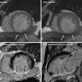
Fig. 2
Example of retrospective gating without tube current modulation. Short-axis (left), two-chamber (middle), and four-chamber (right) views of the heart at end-diastole (top row) and end-systole (bottom row). With full current delivered at both time points, there is no difference in image quality between the two sets of images. This technique results in a higher radiation dose. An example ECG tracing without tube current modulation is shown demonstrating a sustained acquisition over multiple heartbeats
2 Technique
2.1 Retrospective Acquisition
In order to extract functional data from a cardiac CT exam, the heart must be imaged in both end-systole and end-diastole. To ensure that the appropriate cardiac phases are imaged, retrospective gating is usually performed. With this technique, a sustained current is generated by the X-ray tube to image throughout the cardiac cycle, during which time the table moves continuously, resulting in a helical acquisition. A low pitch is used in order to image each part of the heart throughout the R–R interval. A simultaneous ECG tracing is obtained corresponding with the image data. This differs from the prospective-triggered axial acquisition in which the tube current is only on during a pre-specified portion of the cardiac cycle, and the table moves in a step-and-shoot fashion. In addition to evaluating cardiac function, retrospective gating is helpful in evaluating patients who have arrhythmias or who are prone to premature or dropped beats because it allows reconstruction of any phase of the cardiac cycle.
ECG-modulation during a retrospectively gated acquisition may be used to reduce the radiation dose. ECG-modulation allows the user to use full current during a certain pre-defined phase of the cardiac cycle, for example between 45–70 % of the R–R interval. During the remaining phases, the tube current is reduced to a pre-specified level (usually 20 % of the maximum, but the level is customizable on some scanner models) (Fig. 3). ECG-modulation with MinDose (Somatom Definition, Siemens Medical Solutions, Germany) reduces this baseline current further to just 4 % (Fig. 4). The reduction in radiation dose depends on the width of the pulse window chosen to deliver the maximum radiation and on the amount of current delivered at baseline. Approximately 40–60 % reduction in radiation dose can be realized using these techniques (Hausleiter et al. 2006, 2007).
Fig. 3
Example of retrospective gating with tube current modulation. Short-axis (left), two-chamber (middle), and four-chamber (right) views of the heart at end-diastole (top row) and end-systole (bottom row). Notice the difference in image noise at end-diastole, obtained at full tube current, and end-systole, obtained at 20 % of maximum tube current. Despite the increased image noise at end-systole, images are adequate for delineation of endocardial contours for functional measurement. An example ECG tracing with tube current modulation at 20 % is shown
Fig. 4
Example of retrospective gating with tube current modulation down to 4 % of the maximum current. Short-axis (left), two-chamber (middle), and four-chamber (right) views of the heart at end-diastole (top row) and end-systole (bottom row). There is significant difference in image noise at end-diastole at full tube current and end-systole, obtained at 4 % of maximum tube current. Despite the increased image noise at end-systole images are quite adequate for delineation of endocardial contours for functional measurement in this relatively thin patient. An example ECG tracing with tube current modulation at 4 % is shown
2.2 Implication of Scanner Type
Using modern 64-slice MDCT with retrospective gating, a continuous helical scan is obtained over multiple heartbeats with coverage of the entire heart. Due to the retrospective technique, a low pitch is used, creating regions of oversampling. Newer scanners with expanded z-axis coverage, such as 320-slice MDCT (Aquilion One Dynamic Volume CT, Toshiba Medical System, Tochigi-ken, Japan), have a detector width of 16 cm allowing a single-heartbeat acquisition. Dual-flash imaging with DSCT during end-systole and end-diastole has been offered as a potential method to obtain functional data without using retrospective gating, with significant reduction in radiation dose. This technique, however, is rarely used in clinical practice and is still under investigation.
2.3 Beta Blockers
Most studies performed for evaluation of the coronary arteries employ the use of beta-blockers to reduce the heart rate for improved image quality. A target heart rate in the high 50 to low 60 s is required for most scanners. While beta-blockade has been shown to improve the diagnostic image quality of the coronary arteries, there is evidence to suggest there are concurrent effects on left ventricular function. A study by Port using echocardiography demonstrated a reduction in ejection fraction in healthy adults after administration of propranolol (Port et al. 1980; Mo et al. 2011). The proposed mechanism is that through negative inotropic action on the heart, ESV increases, thus decreasing the EF. Other studies in healthy patients using cardiac CT for measurement of left ventricular function show similar results, although differences in ESV and EF were modest (Mo et al. 2011).
Studies in patients with heart disease have shown that beta-blockade can produce decreases in measured function, again resulting from increases in ESV (Dell’Italia and Walsh 1989; Jensen et al. 2010). Because most cardiac CTAs performed today are for evaluation for coronary artery disease, the use of beta-blockers for improving image quality usually takes precedence over potential fluctuations in measured LVEF. Scanners with improved temporal resolution (up to 73 ms) have precluded the need for beta-blockade in many patients, particularly when retrospective gating is utilized.
2.4 Contrast Injection
Depending on the cardiac chambers of interest, the injection parameters may require modification from a traditional coronary CTA. Typical coronary CTA employs either bolus tracking or test bolus technique to measure the transit time of the contrast from the site of injection to the ascending aorta. Many institutions utilize a saline chaser after injection of contrast medium. This results in a tighter contrast bolus and reduces streak artifact in the central veins of the thoracic inlet. This technique provides high contrast opacification of the coronary arteries and adequate delineation of the LV endocardium.
In order to achieve adequate, reliable, contrast opacification of both the RV and LV, a multiphasic injection is needed. This involves contrast injection at a normal flow rate (4–7 cc/sec) to opacify the left heart followed by a slower rate (2–4 cc/sec) to opacify the right heart. This is then followed by a saline chaser. An alternative technique is to first inject contrast and follow with a mixture of contrast and saline in a 60:40 or 50:50 ratio. A typical injection may consist of 50 ml of contrast at 6 cc/sec followed by an additional 50 ml of the contrast/saline mixture at 6 cc/sec. Using a multiphasic technique allows contrast opacification of both the left and the right ventricles and reduces the chance of generating streak artifact from highly concentrated contrast in the SVC, right atrium, or right ventricle (Gao et al. 2012). Lee et al. (2012) analyzed the accuracy of CT in measuring RV function using automated processing software and compared the results to CMR. Low attenuation of the RV blood pool correlated with greater discrepancy with CMR; whereas, when the RV blood pool was greater than 176 HU, measurements were closer to those of CMR, underscoring the importance of proper contrast injection technique.
2.5 Reconstruction Phases
After retrospective scanning, the user has the ability to select the number of phases available for reconstruction. A phase is an interval of the cardiac cycle, usually expressed as a percentage of the RR interval. For example, for reconstruction of cine images, reconstruction of equally spaced phases over the RR interval are obtained, generally in 5 or 10 % increments (yielding 20 or 10 phases, respectively). Increasing the number of phases reconstructed from 10 to 20 doubles the number of images generated for review. A study by Ko et al. (2011) compared 10 and 20 phase reconstruction with respect to cardiac function using a 64-slice scanner. No significant difference in LV volume or EF was observed between the two methods. The increase in the number of phases reconstructed does not change the inherent temporal resolution of the scanner, which is a function of the gantry rotation.
Newer scanners with faster gantry rotation times may be able to take better advantage of more reconstruction intervals. First and second generation dual source CT (DSCT) has the advantage of significantly improved temporal resolution compared to conventional single source CT. Puesken et al. (2008) compared 10 and 20 phase reconstruction using a first generation DSCT. Though use of 20 phases changed the selection of the ES and ED phase in about half of patients, this change resulted in an average 1.9 % change in EF, suggesting that 10 phase reconstruction may be adequate in DSCT as well.
2.6 Post-Processing
One of the major advantages of CT over other modalities is that images are readily acquired as a volumetric dataset. This allows reconstruction of the image in any plane. Modern software packages allow reconstruction of cine images on-the-fly allowing instantaneous visualization of an abnormality in an orthogonal plane. Short axis, 4-chamber, 3-chamber, and 2-chamber views are used to evaluate global function and to evaluate regional wall motion abnormalities. 3-D images of the ventricular blood pool can be obtained with the myocardium subtracted, simulating conventional catheter ventriculography.
2.7 Semi-automatic Versus Automatic Versus Manual
There are multiple methods available to quantify right and left ventricular volumes ranging from time-intensive manual techniques to fully automated software packages. All techniques rely on measurements in end-diastole and end-systole.
The area-length method is a technique borrowed from echocardiography and can be used in calculating left ventricular volume with CT. As the name implies, this technique relies on the measurement of the area and length of the left ventricle. The area is calculated in either the vertical or horizontal long axis plane. The length is measured as the distance from the mitral valve plane to the apex. Using the following formula, left ventricular volume is then calculated.
This formula uses geometric assumptions about the left ventricle, specifically assuming an ellipsoid shape. A variation of the area-length method is the biplane area-length method which uses both the vertical and horizontal long axes to calculate the volume.
Simpson’s method is commonly used in calculating ventricular volume in CMR and can be used to calculate both left and right ventricular volume. In contrast to the area-length method, Simpson’s method does not rely on assumptions about ventricular shape. Using this technique, contours are drawn around the endocardial border in end-systole and end-diastole in the short-axis plane. Each contour represents a volume determined by the slice thickness and gap or overlap. The contours are summed using the following formula where A is the cross-sectional area and S is the slice thickness plus gap, or slice thickness minus overlap.
Studies comparing area-length method and Simpson’s method have shown close agreement between the two, even in patients with regional wall motion abnormalities, although there is slight overestimation of EDV, ESV, and SV using the area-length method (Lessick et al. 2008).
Semi-automated and fully automated software packages are available from multiple vendors. These use a threshold-based segmentation that detects the difference in attenuation between the ventricular chamber and the myocardium; thus, adequate opacification of the blood pool is required. The main advantage of these techniques is the significant time savings over manual processing. A byproduct of semi-automated and fully automated segmentation is that once the mitral valve plane is defined, all available phases can be segmented, allowing time-volume curves to be drawn. Studies comparing manual, semi-automated, and fully automated software have shown close correlation of ventricular volumes using these methods with significant reduction in processing time and good interobserver variability (Greupner et al. 2011; Juergens et al. 2008; Plumhans et al. 2009).
A caveat of the threshold-based methods is that papillary muscles are excluded from the blood pool. This results in systematic underestimation of EDV and ESV as well as overestimation of EF compared to CMR. However, when the same software tools and measurement methods are used for analysis of both the CT and MR, close agreement between the two modalities is observed (de Jonge et al. 2011).
The threshold method is also susceptible to errors from high-attenuation material. For example, streak artifact from dense contrast in the central veins or right heart can lead to errors in contour detection. Pacemaker leads can cause the software to include the right atrial or ventricular chambers in the LV blood pool. Ventricular septal defects can cause similar errors owing to a continuous, unbroken column of contrast (Juergens et al. 2008; van Ooijen et al. 2012).
2.8 Calculation of Values
Once EDV and ESV are acquired, simple subtraction of the values yields the stroke volume (SV); that is, the amount of blood ejected from the ventricle with each beat. Importantly, the SV calculated using this method includes blood flow in any direction, not exclusively flow through the ventricular outflow tract. Regurgitant flow through the mitral or tricuspid valve and ventricular septal defects will be included in this value. As an internal check, and in the absence of valvular regurgitation or shunting, the stroke volume in the RV and LV should be the same.
Cardiac output can then be obtained by multiplying the SV by the heart rate.
The ejection fraction is calculated by determining the percentage of blood exiting the ventricle using the EDV as the baseline.
Normalization of these values to the body surface area (BSA) is helpful to stratify results.
3 Left Ventricle
3.1 Normal Values
Numerous studies have defined the normal values of left ventricular volume using CMR and echocardiography. Because of differences in temporal resolution, image quality, and measurement technique, values obtained with other modalities should not be translated to CT (Lin et al. 2008). Values normalized to BSA are given below.
Normal values for the left ventricle using MDCT | ||||
|---|---|---|---|---|
Parameter | Men | Women | ||
Mean | SD | Mean | SD | |
ESV (ml) | 48.56 | 16.13 | 29.58 | 11.1 |
EDV (ml) | 143.58 | 28.11 | 102.14 | 12.61 |
ESVI (ml/m2) | 24.48 | 8.51 | 17.63 | 6.66 |
EDVI (ml/m2) | 72.35 | 15.09 | 60.86 | 13.31 |
EF (%) | 66.9 | 7.3 | 71.6 | 7.9 |
3.2 Comparison with Echo, MR
The combination of excellent temporal resolution and good spatial resolution make CMR the current gold standard for the evaluation of left ventricular function. Numerous studies have evaluated measurements of left ventricular function using CCT compared with CMR. A meta-analysis of 8–16 slice MDCT compared to CMR demonstrated close correlation of ESV, EDV, and LVEF. The use of multi-segmental reconstruction algorithms showed improvement in correlation, likely owing to increased temporal resolution allowed by these techniques (van der Vleuten et al. 2006).
Current scanner technologies, including 64-, 128-, 256-, 320-slice single source CT, and dual source CT (64 and 128 slice), have also shown excellent correlation with CMR even without the use of multi-segmental reconstruction algorithms due to improvement in temporal resolution.
CT versus MRI | n | CT scanner | EDV | ESV | EF | |||||||
|---|---|---|---|---|---|---|---|---|---|---|---|---|
r | Bias (ml) | SD (ml) | r | Bias (ml) | SD (ml) | r | Bias (%) | SD (%) | ||||
Dual source CT | ||||||||||||
Takx et al. (2012) | 20 | DSCTa | 0.89 | −5.1 | 21.6 | 0.95 | −5.7 | 14.7 | 0.87 | 5.1 | 7.6 | |
Bastarrika et al. (2008) | 12 | DSCT | 0.70 | 16.6 | 18.6 | 0.39 | 4.9 | 6.9 | 0.64 | −0.3 | 3.2 | |
Brodoefel et al. (2007) | 20 | DSCT | 0.98 | −2.2 | 0.99 | −1.4 | 0.95 | 0.7 | ||||
Busch et al. (2008) | 15 | DSCT | 0.81 | 3.7 | 25.4 | 0.79 | −2.6 | 17.3 | 0.64 | 3.8 | 9.4 | |
Jensen et al. (2010) | 32 | DSCT | 0.87 | −1.3 | 17.7 | 0.92 | 1.0 | 8.3 | 0.83 | −1.0 | 4.5 | |
Lunders | 30 | DSCT | 0.96 | −0.3 | 18.2 | 0.98 | 1.1 | 7.8 | 0.97 | −1.1 | 7.8 | |
van der Vleuten et al. (2009) | 34 | DSCT | 0.96 | 11.0 | 54.8 | 0.97 | 3.5 | 31.9 | 0.90 | 0.4 | 4.5 | |
64 SLICE CT | ||||||||||||
Akram et al. (2009) | 20 | 64 | 0.80 | 0.6 | 21.4 | 0.86 | −2.3 | 8.5 | 0.92 | 1.6 | 3.4 | |
Annuar et al. (2008) | 32 | 64 | 0.98 | −8.8 | 12.5 | 0.98 | −6.3 | 9.8 | 0.92 | −2.3 | 6.7 | |
Guo et al. (2009) | 51 | 64 | 0.93 | 5.7 | 27.8 | 0.92 | 0.8 | 17.5 | 0.89 | 1.3 | 5.7 | |
Maffei et al. (2012) | 79 | 64 | 0.59 | 3.3 | 25.8 | 0.76 | 2.6 | 35.1 | 0.73 | 0.6 | 21.1 | |
Sarwar et al. (2009) | 21 | 64 | 0.91 | 0.94 | 0.90 | |||||||
Schlosser et al. (2007) | 21 | 64 | −19.9 | 20.3 | −13.4 | 10.3 | 3.9 | 7.5 | ||||
Wu et al. (2008a) | 41 | 64 | 0.96 | 0.98 | 0.95 | |||||||
Wu et al. (2008b) | 63 | 64 | 0.98 | −0.6 | 15.2 | 0.99 | 1.1 | 10.6 | 0.97 | −0.2 | −4.2 | |
4-16 SLICE CT | ||||||||||||
Belge et al. (2006) | 40 | 16 | 0.92 | 0.95 | 0.95 | |||||||
Dewey et al. (2006) | 88
Related posts: Time-Resolved CT Imaging of Myocardial Perfusion: Dual-Source CT Time-Resolved CT Imaging of Myocardial Perfusion: Dual-Source CT
 Evaluation of the Myocardial Blood Supply: Single-Source, Single-Energy CT Evaluation of the Myocardial Blood Supply: Single-Source, Single-Energy CT
 CT Angiography: State of the Art CT Angiography: State of the Art
 are We Interested in Viability? are We Interested in Viability?
 Myocardial Perfusion Imaging: Clinical Implementation Myocardial Perfusion Imaging: Clinical Implementation
 Evaluation of the Myocardial Blood Supply: Dual-Source Dual-Energy CT Evaluation of the Myocardial Blood Supply: Dual-Source Dual-Energy CT
Stay updated, free articles. Join our Telegram channel
Full access? Get Clinical Tree
 Get Clinical Tree app for offline access

| |||||||||||