Chapter 12 Assessment of Left Ventricular Mechanical Dyssynchrony

Real-time three-dimensional echocardiography (RT3DE) has proven to be the most reliable and reproducible echocardiographic measure of left ventricular volumes, ejection fraction (EF), and mass.^1,² The advent of the matrix array transducer and improvements in parallel processing technologies have improved the temporal and spatial resolution of the volumes acquired, and full left ventricle (LV) datasets can now be obtained in a single heartbeat on some commercial systems.³

Mechanical dyssynchrony, an uncoordinated pattern of left ventricular contraction, has been described in a variety of patient cohorts, including those with left ventricular systolic dysfunction and right ventricular pacing. A reliable and reproducible measure of left ventricular mechanical dyssynchrony has proved elusive, as evidenced by the Predictors of Response to CRT (PROSPECT) study, which demonstrated poor agreement between multiple two-dimensional (2D), M-mode echocardiographic, and tissue Doppler measures of dyssynchrony in patients undergoing cardiac resynchronization therapy (CRT).⁴ The inability to image the entire LV simultaneously also was noted as a drawback to these measures.

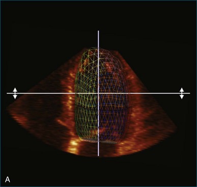
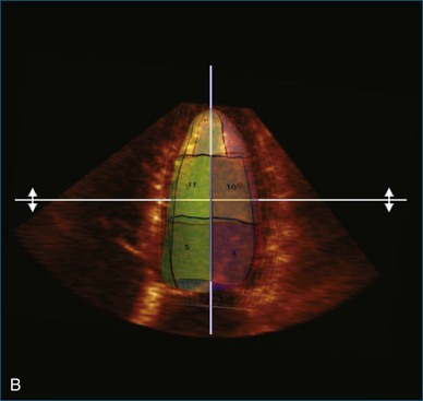
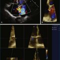
Kapetanakis and colleagues ⁵ proposed RT3DE quantification of regional myocardial function as an accurate measure of left ventricular mechanical dyssynchrony, which might overcome the shortcomings of traditional measures of dyssynchrony. This method is based on the construction of a cast of the LV using semiautomated endocardial border recognition throughout the cardiac cycle. The cast is then segmented into 16 or 17 segments around a central axis, corresponding to American Society of Echocardiology guidelines (Figure 12-1; Video 12-1). Segmental volume or time curves are constructed, and a dyssynchrony index (SDI-16 or SDI-17) is calculated on the basis of the standard deviation of the time to minimal segmental volume as a percentage of the R-R interval (Figure 12-2; Video 12-2). Indexing to the R-R interval allows comparison of the systolic dyssynchrony index (SDI) between subjects with differing heart rates. This method has been validated against cardiac magnetic resonance imaging (MRI) and single-photon emission computed tomography for the assessment of left ventricular dyssynchrony and has been shown to correlate well with other echocardiographic measures of dyssynchrony, such as tissue Doppler.⁶^–⁸

Figure 12-1 Endocardial border detection throughout the cardiac cycle produces a “cast” of the left ventricle, which is segmented according to the American Society of Echocardiography guidelines into either 16 or 17 segments (see Video 12-1).

Figure 12-2 Example of time-volume (A) and normalized volume (B) curves in a patient with normal left ventricle function. The volume curves are U-shaped, and the minimum volume is within a narrow range, suggesting synchronous contraction and a low systolic dyssynchrony index. In this case, the average minimum volume is approximately 50%, suggesting an ejection fraction of roughly 50% (see Video 12-2).

Time and Volume Curves

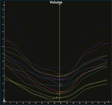
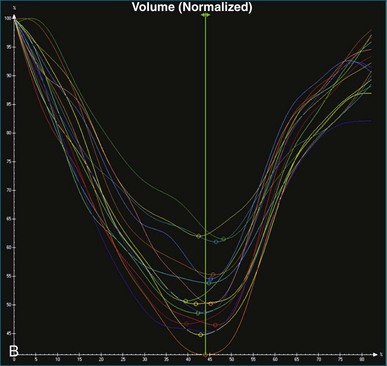
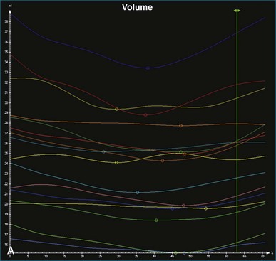
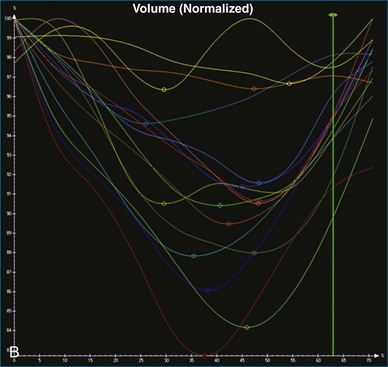
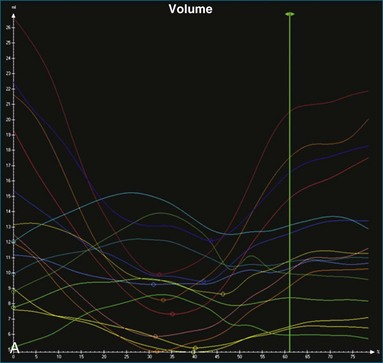
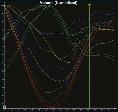
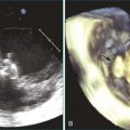
The software for LV analysis produces plots of the absolute segmental volume against time as well as normalized volume curves. When the absolute volumes are normalized such that the greatest volume represents 100%, the difference between 100% and the average of the minimum segmental volumes represents the EF. Segmental volume curves may be viewed individually, but the pattern of segmental contraction is useful and forms the basis of the SDI. The minimum volume point is identified on each curve. In a normal ventricle, the spread of the minimum volume points is narrow, leading to a low standard deviation from the mean time (see Figure 12-2). The volume curves may be used to identify regional wall motion abnormalities due to differences in amplitude between segments (Figure 12-3). A septal flash also is readily identified using the volume curves (Figure 12-4).

Figure 12-3 Time-volume curves in a patient with impaired left ventricular systolic function. A, The time-volume curves are relatively flat, with little change in absolute volume throughout the cardiac cycle, indicating severe left ventricular systolic dysfunction. B, The amplitude of the normalized volume curves is greater, making the minimum volume point easier to identify. The dispersion of the minimum volume points is greater compared with the patient with normal left ventricular systolic function. This indicates a high systolic dyssynchrony index and therefore significant dyssynchrony. The mean minimum volume is approximately 85% of the maximum, suggesting an ejection fraction in the region of 15%.

Figure 12-4 A, In this patient with ischemic left ventricular systolic dysfunction, the time-volume curves are relatively flat, although the U shape of some curves is preserved, suggesting regional wall motion abnormalities. B, When the normalized volume curves are inspected, the minimum volume of the septal and anteroseptal curves (green and light blue curves) occur at the beginning of systole. This is consistent with a septal flash.

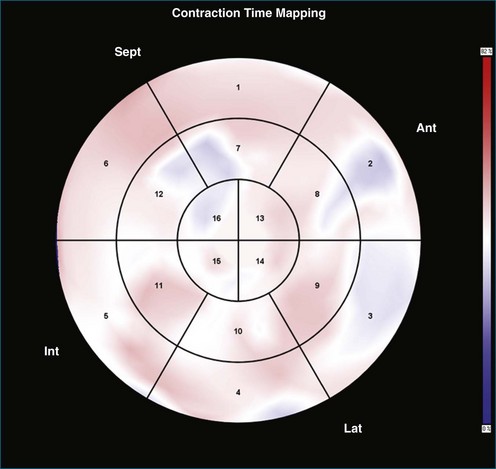
Contraction Front Mapping

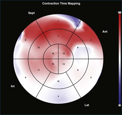
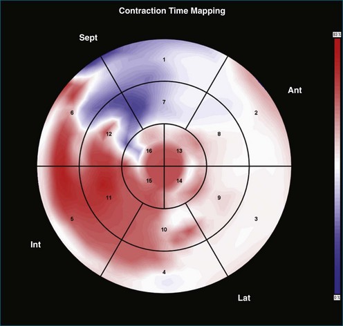
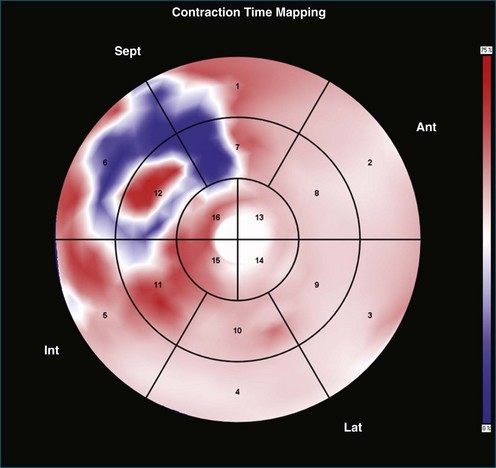
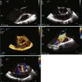
Contraction front mapping analyzes temporal and spatial activation of left ventricular contraction, representing the myocardial segments that reach peak contraction every 25 ms on a color-coded polar map of the LV. As the contraction front spreads through the ventricle, the color changes from red to blue, allowing areas of late contraction to be easily identified. The normal left ventricular activation pattern is homogeneous and rapid (Figure 12-5; Video 12-3). The activation pattern in patients with left ventricular systolic dysfunction is variable, but generally a U-shaped activation pattern is noted (Figures 12-6 and 12-7; Videos 12-4 and 12-5). In our experience, the region of maximal delay most commonly appears to be the septum, leading to a predominant left-to-right color transition. No definite pattern has been established in cases of left bundle branch block, although a septal flash may be identified in some cases (Figure 12-8; Video 12-6). This tool also has been used to identify regional wall motion abnormalities at rest and during stress echocardiography.

Figure 12-5 Normal static map showing homogeneous transition with a large area through white to blue (see Video 12-3). Ant, anterior; Int, interior; Lat, lateral; Sept, septal.

Figure 12-6 Typical static map in a dyssynchronous patient showing U-shaped earliest color transition predominantly in the basal lateral and inferolateral segments, suggesting a predominant left-to-right activation. The activation also is slower than normal; a large part of the map remains red (see Video 12-4). Ant, anterior; Int, interior; Lat, lateral; Sept, septal.

Figure 12-7 Atypical static map showing U-shaped right-to-left activation, with first color transition predominantly in the basal anteroseptal and anterior segments (see Video 12-5). Ant, anterior; Int, interior; Lat, lateral; Sept, septal.

Figure 12-8 A clear septal flash is seen (dark blue). This is again associated with a typical predominant left-to-right transition; the next activation is seen in the basal lateral and inferolateral segments (white) (see Video 12-6). Ant, anterior; Int, interior; Lat, lateral; Sept, septal.

Reproducibility of Systolic Dyssynchrony Index

Excellent reproducibility was noted in the original description of SDI.⁵ The authors described test-retest variability ranging from 1% for end-diastolic volume (EDV) to 4.6% for SDI. Intraobserver variability ranged from 0.6% for EDV to 8.1% for SDI, and interobserver variability ranged from 3.5% for EDV to 6.4% for SDI. The investigators further tested the reproducibility of the technique in a two-center study involving institutions in the United Kingdom and Hong Kong.⁹ To ensure that methods were comparable, a cross-site training program was devised with 20 “training” datasets. The authors reported excellent agreement at the end of the training period. Subsequently, datasets of 62 patients with reduced left ventricular systolic function who were planned for cardiac resynchronization therapy were shared between the two sites and independently analyzed. Intraclass correlation (ICC) coefficients in this study were excellent at greater than 0.8 for all parameters studied (EDV, end-systolic value [ESV], EF, and SDI). Interhospital variability was 2.9% for EDV, 1% for ESV, 7.1% for EF, and 7.6% for SDI.

Soliman and colleagues ¹⁰ elucidated reproducibility further by categorizing dataset quality in 50 randomly selected patients included in their study and noted the reproducibility of SDI to be better in patients with good-quality datasets (interobserver variability of 9% and ICC of 0.99 in patients with good-quality datasets compared with interobserver variability of 16% and ICC of 0.95 in patients with moderate-quality datasets). Overall excellent reproducibility was noted in this study (interobserver variability of 12%, intraobserver variability of 10% for SDI, and both interclass correlation coefficients >0.95).

Normal Values for Systolic Dyssynchrony Index

A number of studies have sought to establish normal values for SDI. On the basis of current evidence, the normal value of the SDI-16 appears to be approximately 3% to 4%, with a maximal value below 6% in normal individuals.^5,¹⁰^–¹⁴ There appears to be a normal apex-to-base contraction gradient, which creates a peristaltic-type contraction pattern in the normal heart.¹²^–¹³ There does not appear to be a significant difference between genders, and SDI does not appear to change significantly with increasing age. A strong negative correlation between SDI-16 and EF has been shown in several studies, and SDI has been demonstrated to be independent of QRS duration.^5,^7,¹²

Clinical Significance of Systolic Dyssynchrony Index

Right Ventricular Pacing

Right ventricular pacing has been shown to increase the SDI and to disrupt the normal apex-to-base contraction gradient of the heart.¹⁵ This is particularly true in patients with right ventricular apical pacing and is associated with a reduction in left ventricular ejection fraction. Baseline reduced left ventricular systolic function and high pacing burden appear to worsen this phenomenon.¹⁶ This phenomenon suggests a potential mechanism for the worsened left ventricular systolic function observed in patients undergoing right ventricular pacing.

Role in Patients with Heart Failure

Dyssynchrony has been found to correlate with reduced exercise capacity in patients with heart failure and left ventricular systolic dysfunction. Dyssynchrony also has been found to correlate with markers of collagen synthesis in patients with tetralogy of Fallot repair. We have postulated increased collagen synthesis or fibrosis as a possible mechanism for increased dyssynchrony, leading to reduced left ventricular systolic function.

Predicting Response to Cardiac Resynchronization Therapy and Assessing Response

Several studies have determined that patients with a high SDI are more likely to benefit from CRT than are those with a lower SDI. In addition, SDI has been found to decrease in those who respond well to CRT but appears to remain unchanged or even worsen in nonresponders.

Several studies have shown responders to have a significantly higher baseline SDI and a significantly greater acute drop in SDI after biventricular (BiV) pacemaker implantation. In patients with CRT devices, RT3DE has been used to demonstrate acute changes in left ventricular volumes, EF, and SDI between the CRT-on and CRT-off modes. SDI-16 has been shown to predict response to CRT in single-center studies.¹⁷^–²⁰ The regional volume curves generated allow identification of the latest contracting segment. There is evidence that siting the left ventricular pacing lead as close as possible to the latest contracting segment provides incremental benefit.²¹ There is emerging evidence that persistently elevated SDI after CRT can identify a subpopulation of patients who will benefit from device optimization.

Technique for Left Ventricle Analysis

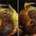
LV analysis may be performed with a number of software packages, all following similar principles, although the results are not directly comparable due to differences in methodology and software algorithms. Described are the steps of LV analysis using 4D LV Analysis software (TomTec, Munich, Germany).

1. The end-systolic and end-diastolic frames are identified, and the axis of the LV is identified using the apex and mitral valve annulus as landmarks (Figure 12-9; Video 12-7).

2. The endocardial border is identified at end systole and end diastole in three cut frames corresponding to the traditional 2D apical views (four-chamber, two-chamber, and long-axis views). This is performed in the same manner as Simpson’s biplane view, excluding the endocardial trabeculae and papillary muscles. There is usually a tradeoff between the accuracy of estimated volumes compared with MRI and accuracy of tracking. Placing the border more subendocardially to mid-myocardially improves the correlation between 3D echocardiography and MRI volumes. However, this may be at the cost of accurate tracking, leading to a less accurate SDI. Our practice is initially to place the borders further out. However, if tracking proves inaccurate, we move the border closer to the blood-tissue interface (Figure 12-10; Videos 12-8 to 12-10).

3. These data are then used to generate a model of the LV throughout the cardiac cycle using endocardial border detection software (see Figure 12-1). The model is inspected to ensure accurate identification of the endocardial border and reliable tracking throughout the cardiac cycle. This is done in the short-axis and again in the long-axis views. This step is particularly important because accurate border tracking is essential for identification of the exact timing of the end-systolic subvolumes (Video 12-11).

4. If necessary, tracking may be adjusted in a number of ways (Figure 12-11). Initially, the contour detection sensitivity may be adjusted. This step makes the model more “stiff” because it increases dependence on the user-defined planes (Video 12-12). If tracking remains suboptimal, we return to the endocardial border identification stage and adjust the initial cut plane borders in regions where tracking is poor. It sometimes is necessary to define the border closer to the blood-tissue interface, although this does decrease the accuracy of the volume measurements (Video 12-13). Alternatively, the tracking may be adjusted on the Beutel model on a frame-by-frame basis. This method can increase the jerkiness of the Beutel model that is generated, again making the minimum volume more difficult to identify. This difficulty can be overcome by the “smoothing” function (Video 12-14).