1 s) makes it difficult to perform causal inference based on the past. Consequently, lag-based methods for computing directed interactions are not suitable for fMRI data analysis.
Instead of relying on time lag information, an alternative approach is to compute directed measures based on the joint distribution of time series measured in two or more regions of interest (ROIs). For example, Patel et al. [14] have used a pairwise conditional probability approach (referred to as the Patel tau measure) to study the relative difference between P(Y|X) and P(Y), and conversely, the relative difference between P(X|Y) and P(X), where X and Y denote the activation of two voxels or ROIs in a brain volume. Large differences indicate strong effective connectivity between the two voxels. Given strong effective connectivity between the two voxels, this metric is a measure of ascendancy between X and Y as determined by the ratio of their respective marginal activation probabilities. Specifically, for two connected voxels X and Y, X is said to be ascendant over Y whenever the marginal activation probability of X is larger than that of Y. Another non lag-based technique is the use of Bayesian networks, which rely on multivariate conditional probability distributions to measure effective connectivity [13, 20]. A comprehensive review and comparison of effective connectivity techniques for fMRI data analysis is presented in [18], where it has been noted that non lag-based methods such as the Patel tau measure and Bayesian networks are best suited for effective connectivity analysis of fMRI data [2]. A limitation of Bayesian networks is that most techniques restrict the network topology by assuming the directed graph to be acyclic. Also, the Patel tau measure is limited in the sense that it is a bivariate measure and there are no known extensions to multivariate data. Another limitation of the Patel tau measure is that it cannot be applied directly to continuous-valued random variables.
In this paper, we present a method for directed graphical modeling of brain networks based on a notion of necessity. The ideas of logical necessity and sufficiency were emphasized by Mill [12] in his “method of difference” and “method of agreement” to explain the relationship between random events. These ideas have recently been extended to fuzzy sets by Ragin [15]. In contrast to these works, our method is based on the classical theory of random variables. Our necessity measure is independent of time lag and has some similarity to the Patel tau measure, but can work directly with continuous-valued random variables.
First, we present our model of necessity using an illustrative example. We then extend the definition of necessity to partial necessity, which can deal with multivariate data and is able to distinguish between direct and indirect relationships in a brain network. The proposed necessity measures were applied to resting state fMRI data from the Human Connectome Project (HCP) database.
2 Materials and Methods
2.1 Mathematical Formulation of the Necessity Measure
In this section, we present the mathematical formulation of the proposed necessity measure. Let us denote two Bernoulli random variables by X and Y. We define the necessity of X to Y by
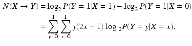
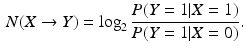 This necessity measure determines the change in the odds of Y being active based on the activation or inactivation of X. The necessity measure takes values on
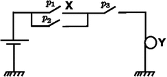
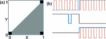
 ![$$\left[ -\infty ,\infty \right] $$](/wp-content/uploads/2016/09/A339424_1_En_31_Chapter_IEq2.gif) . Positive (negative) values indicate that activation of X causes an increase (decrease) in the probability of activation of Y. The magnitude of the necessity value indicates the extent of the increase or decrease in this probability. For example, a necessity value of 1 means that activation of X causes the probability of activation of Y to double. The motivating example for this definition of necessity is a configuration of switches and lamps as shown in Fig. 1. The positions of the switches are modeled as Bernoulli random variables, with
. Positive (negative) values indicate that activation of X causes an increase (decrease) in the probability of activation of Y. The magnitude of the necessity value indicates the extent of the increase or decrease in this probability. For example, a necessity value of 1 means that activation of X causes the probability of activation of Y to double. The motivating example for this definition of necessity is a configuration of switches and lamps as shown in Fig. 1. The positions of the switches are modeled as Bernoulli random variables, with  ,
,  ,
,  indicating the probabilities of these switches being on. The necessity of switch X for activation of lamp Y is given by
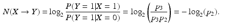 This value is consistent with the intuition: when
  (i.e. the switch in parallel to switch X is always off), the switch X becomes totally necessary for activation of the lamp Y as indicated by
 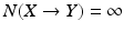 , while when
  (i.e. the switch in parallel to switch X is always on), the switch X becomes unnecessary for activation of Y as indicated by
 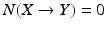 . Note that in this example, the necessity value cannot be negative since
  takes values on [0, 1].
. Positive (negative) values indicate that activation of X causes an increase (decrease) in the probability of activation of Y. The magnitude of the necessity value indicates the extent of the increase or decrease in this probability. For example, a necessity value of 1 means that activation of X causes the probability of activation of Y to double. The motivating example for this definition of necessity is a configuration of switches and lamps as shown in Fig. 1. The positions of the switches are modeled as Bernoulli random variables, with , , indicating the probabilities of these switches being on. The necessity of switch X for activation of lamp Y is given byFig. 1.
An illustrative example of three switches and a lamp motivating the definition of the proposed necessity measure.
(i.e. the switch in parallel to switch X is always off), the switch X becomes totally necessary for activation of the lamp Y as indicated by , while when (i.e. the switch in parallel to switch X is always on), the switch X becomes unnecessary for activation of Y as indicated by . Note that in this example, the necessity value cannot be negative since takes values on [0, 1].Next, we extend this definition to continuous-valued random variables taking values in the [0, 1] interval. For this purpose, we perform the following algebraic manipulation in the discrete-valued case:
 Extending this to continuous-valued random variables with range [0, 1], we get
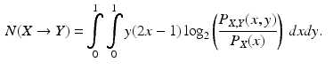
(1)
2.2 Partial Necessity Measure
Note that the necessity metric is a bivariate measure, and therefore in multivariate scenarios (i.e. involving more than two random variables) it does not distinguish between direct and indirect necessity. For example, if X is necessary for Y and Y is necessary for Z, then in this bivariate measure X is also necessary for Z, even though the necessity of X to Z is only indirect (or inherited). In order to study the necessity relationships of two random variables after conditioning on the remaining variables in a multivariate scenario, we introduce the following notion of partial necessity, analogous to the partial correlation measures used in undirected networks. Let  be a set of random variables. The partial necessity of X to Y is denoted as
  where
where 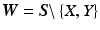 represents the remainder of the random variables, and is given by:
 Note that in this formulation, numerical implementation of the partial necessity measure involves computation of the multivariate integration over
  . This can be computationally expensive if the number of variables involved is large. In order to simplify the computation, we approximate the expectation by the sample mean as follows:
where  indicates the
  sample of
  , and T represents the number of samples. Note that we first perform kernel density estimation to compute the multivariate distribution of
  using all of the samples and then compute the conditional distributions at
  (i.e. at each sample value). This formula is more computationally tractable because it eliminates the
  term, and as a result, avoids the high-dimensional multivariate integration over
  . Note that in multivariate kernel density estimation, there is an exponential increase in the number of samples as the number of dimensions increases (referred to as the “curse of dimensionality”) [9]. However, in this paper, we are dealing with two-dimensional conditional distributions, which may reduce the sensitivity of our measures to increases in the number of variables (or nodes in a network) relative to the full multivariate distribution, an issue we plan to explore further.
be a set of random variables. The partial necessity of X to Y is denoted as where represents the remainder of the random variables, and is given by:. This can be computationally expensive if the number of variables involved is large. In order to simplify the computation, we approximate the expectation by the sample mean as follows:(2)
indicates the sample of , and T represents the number of samples. Note that we first perform kernel density estimation to compute the multivariate distribution of using all of the samples and then compute the conditional distributions at (i.e. at each sample value). This formula is more computationally tractable because it eliminates the term, and as a result, avoids the high-dimensional multivariate integration over . Note that in multivariate kernel density estimation, there is an exponential increase in the number of samples as the number of dimensions increases (referred to as the “curse of dimensionality”) [9]. However, in this paper, we are dealing with two-dimensional conditional distributions, which may reduce the sensitivity of our measures to increases in the number of variables (or nodes in a network) relative to the full multivariate distribution, an issue we plan to explore further.2.3 Interpretation and Properties of the Necessity Measures
In the previous section, a mathematical formulation of the necessity measures was presented. The purpose of this section is to provide an intuitive interpretation and discuss several interesting properties of these measures.
Let X and Y be two binary random variables. In terms of Boolean logic, when X is necessary for Y, Y must be zero whenever X is zero. This condition limits the support of the joint distribution of the two random variables, as illustrated in Fig. 2(a). The black squares represent the support of the joint distribution in the binary-valued case. We can see that the condition that X is necessary for Y requires cases to exist at the bottom-left corner and that no cases may exist at the upper-left corner. Note that when X is one, Y may either be zero or one, as indicated by the presence of black squares in the lower-right and upper-right corners, respectively. Generalizing these statements from binary to continuous-valued random variables results in the joint distribution denoted by the shaded triangle in Fig. 2(a).
 Stable Overlapping Replicator Dynamics for Multimodal Brain Subnetwork Identification
 Transfer Segmentation
 Method to Discover Genetically Driven Image Biomarkers
 Segmentation and Registration Through the Duality of Congealing and Maximum Likelihood Estimate
 Tumor Growth Prediction with Multiplicative Growth and Image-Derived Motion
 Frames for Heart Fiber Reconstruction


Related posts:
Stable Overlapping Replicator Dynamics for Multimodal Brain Subnetwork Identification
Transfer Segmentation
Method to Discover Genetically Driven Image Biomarkers
Stay updated, free articles. Join our Telegram channel
Full access? Get Clinical Tree
