Fig. 1.
Schematic of cable connections between PicoTREC box, MAC box, AFM Controller, and AFM Head Electronics box.
2.
Turn on the AFM controller, MAC box, computer, lamps, and other major electronics and allow them to warm up for at least 30 min in order to minimize the drift of electrical signals during the experiment.
3.
Use the stepper motor to move the sample plate, ensuring that there is enough distance (1.5–2 mm) between the sample plate and the AFM scanner. This will prevent a sudden breakage of the AFM cantilever during the further mounting.
4.
Prior to the mounting of a cell probe, place some reflective material, such as a gold-coated mica or aluminum sheet, onto the sample plate and cover it with a mica sheet. Mount the glass slide with fixed cells on the sample plate, carefully fix the liquid cell with two clips on the glass slide and fill it immediately with ∼650 μL HBSS with Ca2+. Take care that the cells never dry out. Finally, mount the sample plate with the cell probe in the AFM.
5.
Carefully mount the functionalized AFM cantilever on the AFM scanner, taking care that the cantilever will be not dried.
6.
Orient the scanner, mount it onto the microscope stage, fix, and plug it in. Check with a CCD camera to ensure that the cantilever has not broken during the scanner mounting. If any air bubbles are observed, remove the scanner, carefully blot dry with the corner of a filter paper, and then repeat step 6.
7.
Set up the instrument for MAC Mode.
8.
Ensure that the TREC servo on the front of the PicoTREC box is in the OFF position.
9.
Choose an appropriate calibration file for the AFM scanner.
10.
Set one image channel to “Topography” (both in trace and retrace direction) and a second channel to “Aux In BNC” (both in trace and retrace direction) (see Note 12).
11.
MACmode AFM has the advantage over acoustically driven cantilevers that the magnetically coated cantilevers are directly excited by an external magnetic field. This results in a sinusoidal oscillation with a defined resonance frequency. Perform a frequency sweep by tuning the functionalized MAC Lever far away from the sample surface (∼60 μm), choose (Fig. 2) and set the starting drive amplitude (the amplitude meter on the MAC box should read ∼6 V (MAC1.2 box) or ∼1.5–2 V (MACIII box)) (see Note 13).
Fig. 2.
Typical amplitude-frequency (resonance or tuning) curve acquired in buffer (HBSS) with an MAC Lever. Tuning curves were recorded by varying the excitation frequency from 5 to15 kHz; tip-sample separation distance was 60 μm. A distinct resonance peak is obtained at ∼9.3 kHz (using a cantilever with a nominal spring constant of 0.15 N/m). A frequency of ∼8 kHz is used as excitation frequency for imaging (indicated by an arrow ).
12.
Perform a rough approach to the surface. Withdraw the tip and place the tip over a cell of interest with the help of the CCD camera. Adjust the drive signal to attain typically either ∼6 V on the MAC1.2 box or ∼1.5–2 V on the MACIII box.
13.
Approach the sample surface and begin imaging a whole cell (typically at a scan size of ∼60 × 60 μm2). Since VE-cadherin is cell specific and located at intercellular junctions (12, 26), collect AFM data on the contact region between adjacent cells. Topography images (Figs. 3 and 4a) typically illustrate complex filamentous networks with a wide range of forms, likely representing filaments of F-actin and some globular features as well.
Fig. 3.
Typical AFM topographical images (a, b) recorded on gently fixed MyEnd cells.
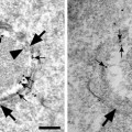
Fig. 4.
Simultaneously recorded Topography (left ) and RECognition (right ) images on vascular endothelial cells with VE-cadherin-Fc functionalized tip. RECognition map of VE-cadherin domains (black spots) represents an amplitude reduction due to a specific binding between VE-cadherin cis-dimers on the AFM tip and VE-cadherin molecules on the cell surface.
14.
Consequently reduce the scanning area to ∼2 × 2 μm2 (Fig. 4). Use a maximum lateral scan speed of ∼3 μm/s; this will result in a total recording time of ∼12 min per image (with a resolution of 512 lines per image). Scan using gain settings as high as possible, but without producing excessive noise. Start with a very low imaging force (high amplitude set-point so that the tip slightly touches the surface; one can check this by opening the “real time cross-section” window and follow the topography cross-section in trace and retrace), and consequently reduce the amplitude set-point to get a fairly good overlay of trace and retrace cross-section lines. Try not to reduce the set-point further; this can cause a strong cross-talk of topography information into the recognition image (27). Setting the proper imaging amplitude is critical (27): it must be large enough to stretch the PEG linker, slightly deflect the cantilever as it oscillates over the target molecule, and detect the binding interactions. Nevertheless, the oscillation amplitude should remain small enough so that the binding does not rupture on each oscillation. Therefore, an imaging amplitude of ∼8–15 nm (this typically corresponds to ∼1.5–2.5 V on the amplitude meter of the MAC1.2 box) is recommended for TREC imaging (see Subheading 3.4 to determine the free oscillation amplitude in nm). Generally, the proper amplitude regime for the observation of recognition events differs from one functionalized cantilever to another, depending upon the length of the linker molecule, on the exact location of the linker molecule on the tip apex, and the size of the attached molecule. Therefore, actual settings will vary, and you might have to change the drive amplitude and approach again.
15.
Recognition is observed as dark “hot” spots in the “Aux in BNC” image channel (Fig. 4 right). Normally the recognition maps of VE-cadherin domains remain unchanged during 1 h of continuous scanning. If no recognition signal is visible after adjusting the gains and amplitude after several frames of images, the functionalized MAC Lever may need to be replaced. It is recommended to functionalize as many MAC Levers as possible (a minimum of 5) to ensure at least one “good” MAC Lever for TREC imaging.
16.
Perform the blocking experiment. Inject 5 mM EDTA very slowly (∼50 μL/min) into the fluid cell while scanning the sample. The first scan after injection might not reveal immediate changes in the recognition map. After 2–3 scans, the recognition spots will practically disappear (Fig. 5 right) as the active VE-cadherin-Fc cis-dimers on the AFM tip dissociate in inactive monomers, thereby abolishing specific VE-cadherin trans-interaction. After blocking experiments, simultaneously recorded topography images should remain unchanged (Fig. 5 left)—indicating that the blocking does not affect membrane topography (see Note 14).
Fig. 5.
Blocking experiment with 5 mM EDTA. Topography (left ) remained unchanged, whereas the recognition clusters practically disappeared in Ca2+-free conditions (right).
17.
To have an additional check on the specificity of the recognition events, the oscillation amplitude should be varied (27). A decrease of the amplitude should result in lower contrast of the recognition spots, since the linker is less stretched. An increase of the amplitude should lead to a sudden disappearance of the recognition spots, since the ligand is no longer able to bind continuously to the receptor’s binding sites. To perform such an experiment, vary the drive amplitude, but maintain the ratio of set-point amplitude to free amplitude.
3.4 Determination of the Free Oscillation Amplitude
The oscillation amplitude should be determined on solid surfaces such as mica or glass.
1.
Open the spectroscopy window. Approach to the surface. Perform a complete amplitude-distance cycle (put Limit to OFF; control the z-piezo limits to not crash the tip) (Fig. 6). The distance between first contact and zero amplitude reflects the peak-to-peak amplitude of free oscillation, providing the ratio of nm/V conversion.
Fig. 6.
Amplitude-distance curve acquired in buffer on a glass slide with an MAC Lever. Trace (light grey line ) and retrace (black line ) are collected using the same cantilever as in Fig. 2.
2.
Adjust the drive signal and the set-point to attain a peak-to-peak set-point amplitude of ∼8–15 nm (corresponds to ∼1.5–2.5 V on the MAC1.2 box). This determined value of the amplitude is the proper setting, which should be used for TREC.
3.
 Histochemical Detection of Lipid Droplets in Cultured Cells
Environmental Scanning Electron Microscopy Gold Immunolabeling in Cell Biology
Histochemical Detection of Lipid Droplets in Cultured Cells
Environmental Scanning Electron Microscopy Gold Immunolabeling in Cell Biology
 Colocalization Analysis in Fluorescence Microscopy
 Morphological Analysis of Autophagy
 A Novel Combined Imaging/Morphometrical Method for the Analysis of Human Sural Nerve Biopsies for Clinical Diagnosis
 Environmental Scanning Electron Microscopy in Cell Biology


Related posts:
Histochemical Detection of Lipid Droplets in Cultured Cells
Environmental Scanning Electron Microscopy Gold Immunolabeling in Cell Biology
Colocalization Analysis in Fluorescence Microscopy
Morphological Analysis of Autophagy
Environmental Scanning Electron Microscopy in Cell Biology
Stay updated, free articles. Join our Telegram channel
Full access? Get Clinical Tree
