Fig. 1.
Experimental setup used for controlled-humidity imaging. The AFM is placed inside a hood to isolate it from the laboratory environment. The humidity is raised and lowered by the addition of a beaker of water or desiccant, respectively. The humidity inside the hood is measured using a digital hygrometer.
2.
Place a beaker of desiccant or water on the control chamber base. Adding a little water, i.e., 10 ml, will probably result in a value of relative humidity (RH) lower than 90%. If 50 ml or more of water at room temperature is added the value of RH will get closer to 95% or more in 0.5–2 h of exposure. The rate at which a given RH is obtained depends on the volume of the control chamber and the amount of water/desiccant added to the beaker. In our experiments we typically use a chamber of approximately 0.01–0.02 m3 (Fig. 1). If a constant value of RH is required, the beaker can be filled with a saturated salt solution. Different soluble salts give rise to different vapor pressures in the chamber. Since conventional AFM imaging is slow, we use pure water, because the RH does not change by more than 1% during acquisition of an image.
4.
Place the lid on top of the chamber’s control base.
6.
The hole into which the digital hygrometer fits should be insulated preventing vapor to leave or enter the chamber.
7.
Use the digital hygrometer to monitor the humidity and also, if required, the temperature. Wait until the relative humidity reaches the appropriate value and stabilizes. With stability here we imply that the relative humidity has reached a steady state where its value does not fluctuate more than approximately 1–2% during the experimental run (see Note 2).
3.3.2 Biomolecular Studies in Ambient AM AFM with Humidity Control
1.
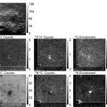
By following the procedures discussed in the previous section, first set a relatively low value of relative humidity RH (Fig. 2a) by placing a given amount of desiccant in the chamber (see Subheading 3.3.1).
Fig. 2.
Summary showing typical conformational changes in closed-circular supercoiled DNA as the humidity is increased, with a corresponding increase in the thickness of the surface water layer. Topological rearrangements in the DNA are observed to induce DNA condensation, kinking of the backbone, and changes in the backbone trajectory. A number of these changes are highlighted with arrows. Reproduced from ref. 43 with permission from the PCCP Owner Societies.
2.
3.
To observe humidity induced topographic rearrangements of the DNA molecule the relative humidity in the chamber should be increased (Fig. 2b, d). This is achieved by first disengaging the tip from the surface while maintaining the lateral xy-piezo position. Then the desiccant is replaced by a beaker of water or saturated salt solution (Subheading 3.3.1).
4.
When the relative humidity has reached a steady state at RH = 95% or above (Fig. 2c, d), take another image of the molecule that has been previously imaged at a low value of RH (see Note 30). Now topologically induced rearrangements of the DNA molecule should be observed to induce DNA condensation, kinking of the backbone, and changes in the backbone trajectory (see Note 3) (43).
3.4 Amplitude Modulation Imaging (Tapping Mode)
3.4.1 Introduction to Amplitude Modulation (Tapping Mode) Imaging
Historically, AM AFM has been the main AFM technique applied to biological systems since its invention (5, 25). The first image of single DNA molecules with a Scanning Probe Microscope (SPM) was obtained by Binnig et al. (44) in 1984 with an STM, before the AFM was invented (4). Since that time, the AFM has been used widely to study biomolecular samples and several good reviews can be found in the literature (1, 4, 10, 13, 14, 26, 29, 30). Nevertheless, in air, the elucidation of the existence and control of the average force per cycle has been one of the main parameters allowing current advances. The average force per cycle can be either attractive or repulsive. If attractive, mechanical contact might still be induced during each cycle but this is minimized (45–48). Tapping mode is typically referred to intermittent mechanical contact, nevertheless, it is now more generally understood as a term to describe standard amplitude modulation (AM AFM) imaging. By standard we imply relatively large values of set-point amplitude A and free amplitude A 0, i.e., approx 0.3 < A/A 0 < 0.95 and 1 < A 0 < 100 nm. In summary, the main results for standard AM AFM imaging are (46):
1.
The average force per cycle might be either net attractive or net repulsive and follows phase shifts above and below 90° respectively. These are the so-called attractive and repulsive regimes.
2.
3.
There might be either one or two physically stable amplitudes for a given cantilever–sample equilibrium position zc. When two solutions exist these are termed the L and H state, where the L state corresponds to the cantilever vibrating at a position higher above the sample. Typically, these two states correspond to the attractive and the repulsive regime.
4.
We can define a critical value of free amplitude A c corresponding to the minimum value of A 0 for which a transition between force regimes might be observed in amplitude–distance (AD) curves. We describe how to find this value in the next subsections below. The main principle is that below and above A c the attractive and the repulsive force regimes prevail respectively (42, 46, 51).
3.4.2 The Attractive and Repulsive Force Regimes
1.
Attractive regime: The attractive force regime is defined as a net attractive average force per cycle where, during one cycle, repulsive forces might or might not be present. It is convention, however, to define the attractive force regime as that for which the phase lag of the cantilever with respect to the drive is larger than 90°. While this convention typically agrees with the above more physically significant definition, there are cases for which it might not (5, 29, 47).
2.
Repulsive regime: The repulsive force regime is defined as a net repulsive average force per cycle where, during one cycle, attractive forces might or might not be present. It is convention, however, to define the repulsive force regime as that for which the phase lag of the cantilever with respect to the drive is less than 90°. While this convention typically agrees with the above more physically significant definition, there are cases for which it might not (see references above).
3.
Amplitude–Phase–Distance (APD) curves: In APD curves the tip–surface separation is slowly decreased and then increased while monitoring the behavior of the amplitude A (AD curves, Fig. 3a) phase Φ (AP curves, Fig. 3b) or both (APD curves). In simulations, other distance curves such as force and contact time distance curves can be acquired. An example of APD curves is given in Fig. 3.
Fig. 3.
(a) Amplitude–distance curve performed on a mica surface at 40% RH for a silicon rectangular cantilever with nominal spring constant of 40 N/m driven at resonance (f 0 ≈ 300 kHz) with a free amplitude A 0 ≈ 10 nm. (b) Corresponding phase–distance curve where a step-like discontinuity is observed as the cantilever goes from the L (attractive regime) to the H (repulsive regime) state when approaching the sample and from the H to the L state during retraction. The path followed is marked from 1 to 7, for the cantilever approach and retraction. The region labeled SASS is a region of the parameter space that typically involves perpetual water contact (29, 42, 54) and is discussed in Subheading 3.7. The free amplitude (A 0) of the cantilever in this example is nearly 10 nm and corresponds to the value of z c when the tip begins to be perturbed by the sample. In air, there is always a 1 to 1 correspondence between amplitude and tip–sample separation, i.e., the amplitude decreases in a linear fashion during approach (notwithstanding the perturbations caused by switching force regimes).
4.
Critical amplitude A c : Force regimes can be monitored experimentally and in simulations via the phase lag (see Table 1 and Fig. 3). Then, the value of A c can be found by acquiring amplitude phase (AP) distance curves (42, 51) and gradually increasing A 0 until the phase lag is observed to lie below 90°, i.e., the onset of the repulsive regime is observed. In Fig. 3 the value of A c has already been reached or surpassed since the repulsive regime is observed to control the interaction on retraction. Thus, in this case, A c < 10 nm. The value of A c typically lies within a range and this range is a consequence of the stochastic nature of the force transitions (42, 52, 53).
Table 1
Outcomes for a hydrophilic tip interacting with a heterogeneous sample, i.e., regions where there is only the mica surface and regions where we have samples such as DNA molecules
A 0 relative to A c | Substrate | Sample (i.e., DNA) | Are water layers perturbed (CT > 0)? | Mechanical contact | ||
|---|---|---|---|---|---|---|
Case | Phase | Case | Phase | |||
A 0 < <1/2A c | W nc | >90º | W nc | >90º | No | No |
A 0 ∼ 1/2A c | W nc | >90º | W c | >90º | Yes | |
W c | >90º | W nc | >90º | |||
W c | >90º | W c | >90º | |||
A 0 ∼ A c | W c | >90º | W c | >90º | ||
Rep. | >90º | W c | >90º | Yes | ||
W c | <90º | Rep. | <90º | |||
Rep. | <90º | Rep. | <90º | |||
A 0> > A c | W c | >90º | Rep. | <90º | ||
Rep. | <90º | W c | >90º | |||
Rep. | <90º | Rep. | <90º | |||
W c | >90º | W c | >90º | No | ||
5.
Example of attractive/repulsive interaction regimes and effects on the topography of a single DNA molecule: Figure 4 shows a sequence of topographic images of a single DNA molecule on mica obtained with the same cantilever-tip used to acquire the APD curve shown in Fig. 3. From a to d, the normalized amplitude set-point (A/A 0) has been systematically reduced from 0.92 to 0.65. The same free amplitude of A 0 (A 0 = 10 nm) as in Fig. 3 for the APD has been used here. Since A c < 10 nm, it is clear that the repulsive regime (H state) should be reached with this value of A 0 only by sufficiently decreasing the set-point amplitude, A. In Fig. 4a, the cantilever is vibrating in the L-state with attractive forces on average. In Fig. 4b, c, there is an unstable region where the cantilever is predominantly in the L-state but transiently switches to the H-state. The H state (repulsive regime) has been stably reached at intermediate values of set-point (Fig. 4d) as predicted by the APD curve in Fig. 3. Both apparent molecular height and width display dramatic differences in the L state (attractive regime) as compared to the H state (repulsive regime). This is also shown in Fig. 5. Note that the noise observed in Fig. 4b, c is not a consequence of an inappropriate choice of integral and proportional gains but a consequence of switching between states (46, 52). That is, even optimization of the feedback gains can be insufficient to induce stability if the cantilever dynamics do not permit one stable oscillation state (55): in these situations no choice of gains makes the noise disappear.
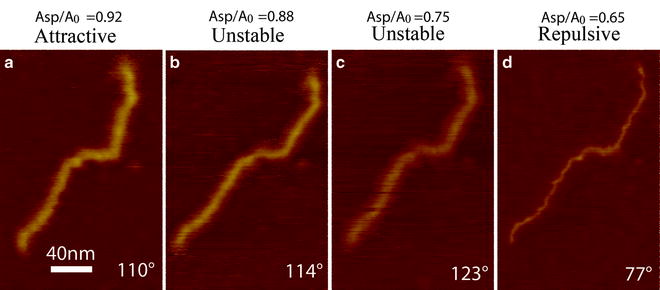
Fig. 4.
Topographic images (Z-piezo signal) of a single 800 bp dsDNA molecule on mica obtained in a sequence where the value of A 0 = 10 nm is larger than the critical value A c (here A c < 10 nm). The average phase shift Φ for every scan is shown on the bottom right in every image and allows differentiating between the L (attractive) and the H (repulsive) state (regimes). Experimental parameters: A 0 ≈ 9 nm, k (spring constant) ≈ 40 N/m, f = f 0 ≈ 300 kHz (drive and natural frequencies), and Q factor ≈ 500.
Fig. 5.
(a) Apparent height and (b) width corresponding to Fig. 4. The L (attractive) and H (repulsive) states (force regimes) and severe bi-stable behavior (B) are differentiated by squares, circles, and triangles, respectively.
3.5 The Effects of the Water Layers on Apparent Height
In the section above we have discussed the effects of varying the free amplitude to reach the attractive and the repulsive force regimes and how these can lead to different degrees of lateral resolution and apparent height of biomolecules. Here, we further distinguish between intermittent water contact and pure noncontact regimes where the water layers on either the tip, the surface (here the mica substrate), or the sample (here the biomolecules) might be disturbed in some cases while in other (pure noncontact mode) might not (42).
Generality can be provided if the concept of critical free amplitude A c is also used here (42, 45, 46, 56). As stated, A c corresponds to the minimum value of A 0 for which a transition between force regimes might be observed in AD curves (see Fig. 3) (46, 51). Recall from above that the force regimes can be monitored experimentally and in simulations via the phase lag (see Table 1). Thus, the A c value for a given sample can be found by acquiring amplitude phase (AP) distance curves (51) and gradually increasing A 0 until the phase lag is observed to lie below 90°, i.e., the repulsive regime (42). We then proceed to define four types of interaction depending on whether the water layers are disturbed on either the mica surface of the sample (i.e., the DNA molecules in this case) and whether the repulsive regime, where intermittent mechanical contact is made, is reached. These four types of interactions can be described generally in terms of A c. See below.
3.5.1 Definition of Interactions Where There Is Water on the Tip and/or the Sample
We write W nc, W c and Rep. for situations where the water layers on the tip are never in contact with the water layers on the sample (W nc), the water layers are perturbed but intermittent mechanical contact does not occur (W c), and Rep. when intermittent mechanical contact between the tip and the sample or surface occurs (i.e., a repulsive interaction). Now we write a convention where the first terms refer to the interaction between the tip and the substrate and the second refers to an interaction between the tip and the biomolecular sample. In this way we write:
1.
W nc/W nc for an interaction where the water layers are never perturbed on either the sample or the substrate (see Table 1).
2.
W c/W c for interactions where mechanical contact does not occur but the water layers are being perturbed. This might also include W nc/W c and other combinations (42).
3.
 Introduction: Nanoimaging Techniques in Biology
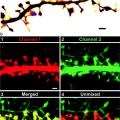 Two-Color STED Imaging of Synapses in Living Brain Slices
 Secondary Ion Mass Spectrometry Imaging of Biological Membranes at High Spatial Resolution
 High Data Output Method for 3-D Correlative Light-Electron Microscopy Using Ultrathin Cryosections
 Functional AFM Imaging of Cellular Membranes Using Functionalized Tips
 Single-Molecule Tracking of mRNA in Living Cells


Rep./W c for interactions where mechanical contact might occur on the sample but not on the substrate. In this case, only the water layers are perturbed on the mica substrate, but this could also occur on the other way around, i.e., W c/Rep. (42).
Related posts:
Introduction: Nanoimaging Techniques in Biology
Two-Color STED Imaging of Synapses in Living Brain Slices
Secondary Ion Mass Spectrometry Imaging of Biological Membranes at High Spatial Resolution
High Data Output Method for 3-D Correlative Light-Electron Microscopy Using Ultrathin Cryosections
Functional AFM Imaging of Cellular Membranes Using Functionalized Tips
Single-Molecule Tracking of mRNA in Living Cells
Stay updated, free articles. Join our Telegram channel
Full access? Get Clinical Tree
