Auto-encoders for Classification of 3D Spine Models in Adolescent Idiopathic Scoliosis

of dimension , representing the 3D coordinates of a spine model, is mapped by an encoder function into the hidden layer $\mathbf {h}$ , often called a code layer in the case of auto-encoders:

$\begin{aligned} \mathbf {h} = f(\mathbf {x}) = s(-\mathbf {W}^{(1)}\mathbf {x}+\mathbf {b}^{(1)})\ \end{aligned}$

(1)

where $\mathbf {W}^{(1)}$ is the encoding weight matrix, $\mathbf {b}^{(1)}$ the bias vector and $s(\cdot )$ the activation function. Note that this one hidden layer auto-encoder network corresponds to a principal component analysis if the activation function is linear. Then, the code representation is mapped back by a decoder function

into a reconstruction $\mathbf {z}$ :

$\begin{aligned} \mathbf {z} = g(f(\mathbf {x})) = s(-\mathbf {W}^{(2)}\mathbf {h}+\mathbf {b}^{(2)})\ \end{aligned}$

(2)

where $\mathbf {W}^{(2)}$ is the decoding weight matrix. Tying the weights ( $\mathbf {W}^{(2)}=\mathbf {W}^{(1)^{T}}$ ) has several advantages. It acts as a regularizer by preventing tiny gradients and it reduces the number of parameters to optimize [2]. Finally, the parameters $\theta =\{\mathbf {W}^{(1)}, \mathbf {b}^{(1)}, \mathbf {b}^{(2)}\}$ are optimized in order to minimize the squared reconstruction error:

$\begin{aligned} L_2(\mathbf {x}, \mathbf {z})=\Vert \mathbf {x} - \mathbf {z} \Vert ^{2}\ . \end{aligned}$

(3)

In the case of dimensionality reduction, the code layer $\mathbf {h}$ has a smaller dimension than the input $\mathbf {x}$ . One major drawback comes from the gradient descent algorithm for the training procedure that is very sensitive to the initial weights. If they are far from a good solution, training a deep non-linear auto-encoder network is very hard [6]. A pre-training algorithm is thus required to learn more robust features before fine-tuning the whole model.

The idea for initialization is to build a model that reconstructs the input based on a corrupted version of itself. This can either be done by Restricted Boltzmann Machines (RBMs) [6] or denoising auto-encoders [18] (used in this study). The denoising auto-encoder is considered as a stochastic version of the auto-encoder [18]. The difference lies in the stochastic corruption process that sets randomly some of the inputs to zero. This corrupted version $\tilde{\mathbf {x}}$ of the input $\mathbf {x}$ is obtained by a stochastic mapping $\tilde{\mathbf {x}} \sim q_{D}(\tilde{\mathbf {x}}|\mathbf {x})$ with a proportion of corruption

. The denoising auto-encoder is then trained to reconstruct the uncorrupted version of the input from the corrupted version, which means that the loss function in Eq. 3 remains the same. Therefore, the learning process tries to cancel the stochastic corruption process by capturing the statistical dependencies between the inputs [2]. Once all the layers are pre-trained, the auto-encoder proceeds to a fine-tuning of the parameters $\theta$ (i.e. without the corruption process).

2.3 K-Means++ Clustering Algorithm

Once the fine-tuning of the stacked auto-encoder has learnt the parameters $\theta$ , low-dimensional codes from the code layer can be extracted for each patient’s spine. Clusters in the codes were obtained using the K-Means++ algorithm [1], which is a variant of the traditional K-Means clustering algorithm but with a selective seeding process. First, a cluster centroid is initialized among a random code layer $\mathbf h$ of the dataset $\chi$ following a uniform distribution. Afterwards, a probability is assigned to the rest of the observations for choosing the next centroid:

$\begin{aligned} p(\mathbf {h})=\frac{D(\mathbf {h})^2}{\sum _{h \in \chi }D(\mathbf {h})^2} \end{aligned}$

(4)

where $D(\mathbf {h})^2$ corresponds to the shortest distance from a point $\mathbf h$ to its closest cluster centroid. After the initialization of the cluster centroids, the K-Means++ algorithm proceeds to the regular Lloyd’s optimization method.

The selection of the right number of clusters

is based on the validity ratio [14], which minimizes the intra-cluster distance and maximizes the inter-cluster distance. The ratio is defined as

. The intra-cluster distance is the average of all the distances between a point and its cluster centroid:

$\begin{aligned} \text{ intra } = \frac{1}{N}\sum ^{k}_{i=1}\sum _{\mathbf {x} \in C_{i}} \Vert \mathbf {h} - \mathbf {c}_{i} \Vert ^{2}. \end{aligned}$

(5)

where

is the number of observations in $\chi$ and $\mathbf {c}_i$ the centroid of cluster

. The inter-cluster distance is the minimum distance between cluster centroids.

$\begin{aligned} \text{ inter } = \min (\Vert \mathbf {c}_{i} - \mathbf {c}_{j} \Vert ^{2}) \end{aligned}$

(6)

where $i = 1, 2,\ldots , k-1$ and $j = i+1,\ldots , k$ .

2.4 Clinical Data Analysis

Once clusters were created from the low-dimensional representation of the dataset, we analyzed the clustered data points with 3D geometric indices in the main thoracic (MT) and thoracolumbar/lumbar (TLL) regions for each patient’s spine. One-way ANOVA tested differences between the cluster groups with a significance level $\alpha =0.05$ . The p-values were adjusted with the Bonferroni correction. For all cases, the following 3D spinal indices were computed: the orientation of the plane of maximum curvature (PMC) in each regional curve, which corresponds to the plane orientation where the projected Cobb angle is maximal; the kyphotic angle, measured between T2 and T12 on the sagittal plane; the lumbar lordosis angle, defined between L1 and S1 on the sagittal plane; the Cobb angles in the MT and TLL segments; and the axial orientation of the apical vertebra in the MT region, measured by the Stokes method [16].

3 Clinical Experiments

3.1 Clinical Data

A cohort of 155 AIS patients was recruited for this preliminary study at our institution. A total of 277 reconstructions of the spine was obtained in 3D. From this group, 60 patients had repeat measurements from multiple clinic visits (mean $$=$$

3 visits). The mean thoracic Cobb angle was $53.2\pm 18.3^{\circ }$ (range $$=11.2$$

– $100.2^{\circ }$ ). All patients were diagnosed with a right thoracic deformation and classified as Lenke Type-1 deformity. A lumbar spine modifier (A, B, C) was also assigned to each observation, using the biplanar X-Ray scans available for each patient. The dataset included 277 observations divided in 204 Lenke Type-1A, 43 Lenke Type-1B and 30 Lenke Type-1C deformities. The training set included 235 observations, while the validation set included 42 observations (15 % of the whole dataset). Observations were randomly assigned in each set.

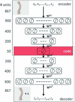
Fig. 1

Illustration of the stacked auto-encoders architecture to learn the 3D spine model by minimizing the loss function. The middle layer represents a low-dimensional representation of the data, called the code layer. An optimal layer architecture of 867-900-400-200-50 was found after a coarse grid search of the hyper-parameters

3.2 Hyper-Parameters of the Stacked Auto-Encoders

The neural network hyper-parameters were chosen by an exhaustive grid search. The architecture yielding to the lowest validation mean squared error (MSE) is described in Fig. 1. We used an encoder with layers of size 867-900-400-200-50 and a decoder with tied weights to map the high-dimensional patient’s spine models into low-dimensional codes. All units in the network were activated by a sigmoidal function $s(a)=1/(1+e^{-a})$ , except for the 50 units in the code layer that remain linear $$s(a)=a$$

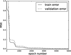
Fig. 2

Evolution of the mean squared error (MSE) with respect to the number of epochs to determine the optimal model described in Fig. 1

3.3 Training and Testing the Stacked Auto-encoders

Auto-encoder layers were pre-trained and fine-tuned with the stochastic gradient descent method using a GPU implementation based on the Theano library [3]. Pre-training had a proportion of corruption for the stochastic mapping in each hidden layer of $v=\{0.15, 0.20, 0.25, 0.30\}$ and a learning rate of $\varepsilon _{0}=0.01$ . Fine-tuning ran for 5,000 epochs and had a learning rate schedule with $\varepsilon _{0}=0.05$ that annihilates linearly after 1,000 epochs. Figure 2 shows the learning curve of the stacked auto-encoder. The optimal parameters $\theta$ for the model in Fig. 1 were found at the end of training with a normalized training MSE of 0.0127, and a normalized validation MSE of 0.0186, which corresponds to 4.79 and 6.46 mm $$^2$$

respectively on the original scale. The learning curve describes several flat regions before stabilizing after 3,500 epochs.