Automated Carotid IMT Measurement and Its Validation in Low Contrast Ultrasound Database of 885 Patient Indian Population Epidemiological Study: Results of AtheroEdge® Software

Fig. 17.1

Samples of high-resolution and low-resolution images. (a) High-resolution image where the intima and adventitia layers are neatly defined, noise is low, and pixel density is high (about 20 pixels/mm). (b) Image acquired by a medium-end scanner without compound imaging, where LI is hypoechoic. (c) Images acquired by a low-end equipment without harmonic imaging and compound, where LI is almost invisible and pixel resolution is very low (about 12 pixels/mm). (d) Example of low-resolution image with high level of image noise

The characteristics that make an image suitable for automated delineation are (see Fig. 17.1) (1) high spatial resolution, (2) high dynamic range, (3) low noise level, (4) compound imaging, and (5) harmonic imaging. When an image has the above-mentioned five characteristics, we can say that it is a high-resolution image and automated IMT measurement algorithms can process it [22, 23]. If the image does not possess one or more of the above-mentioned characteristics, specific image enhancement and delineation or segmentation strategies must be adopted [24]. Compound and harmonic imaging are available on most of the medium-level and high-level ultrasound OEM scanners. However, they are not present in the majority of the entry-level and cheaper equipment so that compound imaging and harmonic imaging are not supported. As a consequence, the image quality becomes low with poor contrast and automated segmentation is difficult and sometimes nearly impossible. As an example, Fig. 17.2 shows three samples of low-resolution images. The left column (Fig. 17.2a, ca, c, e) shows B-Mode longitudinal projections of the images of our low-resolution database. The dashed line represents a region of interest, which is zoomed on the right (Fig. 17.2b, db, d, f). The white arrows indicate where the lack of contrast is more evident. It can be seen that in Fig. 17.2bb, the adventitia layer (MA) is bright, but the intima is sometimes broken and not represented (white arrow). In Fig. 17.2dd, the intima layer cannot be clearly distinguished from the media and adventitia, because all three layers have almost the same gray color. In Fig. 17.2ff, the adventitia is bright, but the intima is almost invisible. These three conditions can represent a very difficult challenge to automated segmentation techniques.

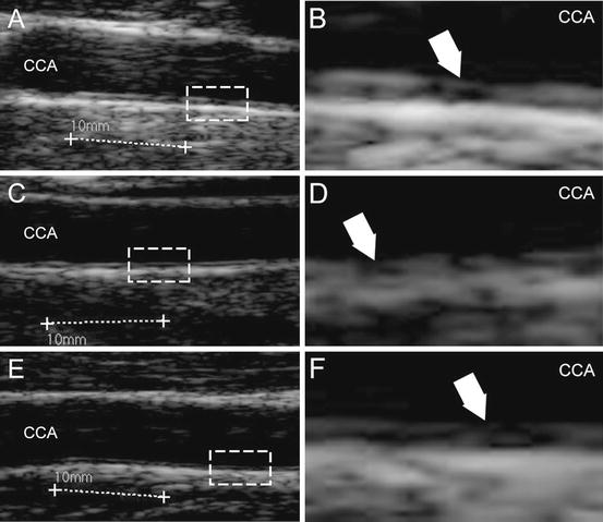
Fig. 17.2

Samples of low-resolution images extracted from the dataset. Panels (a, c), and (e) show the carotid. Panels (b, d), and f show the zoomed portion of the corresponding dashed rectangle on the left. The white arrows indicate the challenges of these images: interrupted intima representation (panel b), low contrast between intima, media, and adventitia (panel d), and well represented adventitia, but hypoechoic intima (panel f)

In this chapter we will present the results of a completely automated epidemiological study devoted to the IMT measurement of healthy subjects from around Hyderabad in India. We used CALEX in its last empowered version 3.0. CALEX3 is a novel and improved technique, which incorporates the rejection of the jugular vein, hard constraints of the seed points, and an optimized fuzzy K-means classifier [25, 26].

2 Image Dataset and Image Characteristics

The database consisted of 885 ultrasound carotid images in longitudinal projection. The subjects for the images were identified through the Hyderabad DXA Study, which included participants drawn from two groups. The first was the participants of the Hyderabad arm of the Indian Migrant Study that included migrants of rural origin, their rural dwelling sibs, and those of urban origin together with their urban dwelling sibs. The second was the participants of the Hyderabad Nutrition Trial which was made up of people born within an earlier controlled, community trial of nutritional supplementation integrated with other public health programs, now aged 18–21. Participants attended screening examination between January 2009 and December 2010, which included assessment of carotid IMT. The study received Ethical Approval by the local Committee of the National Institute of Nutrition and the London School of Hygiene & Tropical Medicine.

The challenging aspect of these images is that they were acquired with low-end ultrasound equipment. Figure 17.3a shows an example of ultrasound B-Mode image. As can be seen, the operator traced calibration lines during the image acquisition. Such lines are 10 mm long. However, such lines are often not horizontally placed, and, therefore, they cannot be used for computing the vertical and horizontal conversion factor independently. The white arrows in Fig. 17.3a indicate the vertical calibration scale. The distance between the white lines indicated by the arrows is 10 mm. We computed the number of pixels between the two white lines and used them to derive the vertical conversion factor. All the images had a vertical pixel density equal to 127 pixels/cm, or 12.7 pixels/mm, which is a very low pixel density that is typical of low-end OEM ultrasound scanners. Therefore, the conversion factor for the images was 0.0787 mm/pixel.

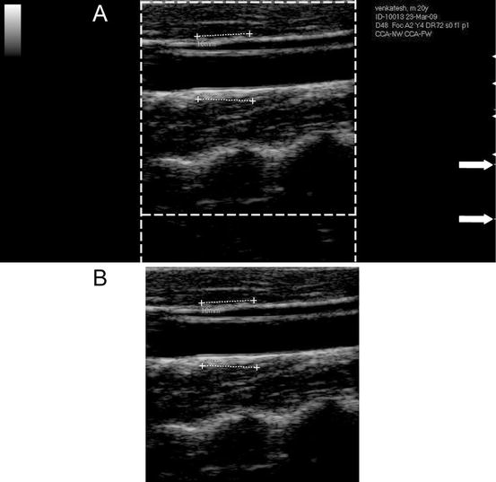
Fig. 17.3

CALEX 3.0 automated cropping. (a) Original image. The dashed lines delimit the region containing the ultrasound data. Outside the dashed lines, the vertical and horizontal gradients are null. The white arrows on the right indicate the vertical scale for the measurement of the conversion factor. (b) Cropped image

All the images were JPEG formatted. In several previous studies, we showed that the black frame surrounding the ultrasound image is detrimental to the automated processing algorithm and must be removed [25–29]. We adopted an automated autocropping strategy we previously published [27]. By computing the horizontal Sobel gradient of the image, we marked the first and last nonzero column, which marked the horizontal extension of the ultrasound data area. By computing the vertical Sobel gradient, we marked the vertical extension of the image area. The result of the automated cropping is shown in Fig. 17.3b.

An expert operator (L.S.) manually traced the far wall LI and MA boundaries by using an ad hoc developed graphical user interface (called ImgTracer™ [30, 31]). As the images were in low contrast and low resolution, the use of ImgTracer™ was justified by zooming the image before tracing. The final LI/MA profiles were saved in numerical form on text file and made available for IMT computation. The manual tracings were considered as ground truth (GT).

3 Brief Architecture of CALEX 3.0

The completely automated technique we used to perform automated IMT measurement was called CALEX (Completely Automated Layers EXtraction). We had previously developed this technique in 2010 [25, 26], but we modified it in order to improve the performance for low contrast and low-resolution carotid ultrasound images. For the purposes of this study, we used the CALEX 3.0 version, which is the latest improvement of our CALEX system architecture. CALEX 3.0 consists of three cascaded stages. Stage-I is the artery recognition phase based on feature extraction, line fitting, and classification [22]. This system was further improved by differentiating the CCA and JV. This was called intelligent carotid artery recognition processor—CALEX 3.0. The output of this stage is the adventitia borders (ADF). Stage-II consists of delineation or segmentation of walls or LI/MA segmentation based on fuzzy K-means classifier for the delineation of the automated LI and MA boundaries. Stage-III consists of LI/MA refinement.

3.1 Stage-I: Automatic Recognition of the CA

Stage-I is based on the pixel analysis through local statistics. The fundamental hypothesis of this recognition stage is that carotid appearance in B-Mode longitudinal images can be modeled in a relatively simple way as a black region (the artery lumen) in between two bright lines, which are the near and far adventitia layers. Therefore, Stage-I of CALEX 3.0 essentially searches for the carotid adventitia layers [25].

First of all, all the local intensity maxima of the images are automatically found and marked. Such maxima are called “seed points.” Seed points are linked to form lines. Figure 17.4a shows the original cropped image and Fig. 17.4b the automatically detected line segments. In all our images, the carotid artery was represented as horizontally placed. Therefore, we kept all the horizontal lines in the image and discarded inclined lines. By using linear discriminators and a very solid classification procedure [32], we detected, among all the line segments, the two that comprised the artery lumen (Fig. 17.4c). The final output of Stage-I is the profiles of the far adventitia layer (AD_F), depicted by Fig. 17.4d.

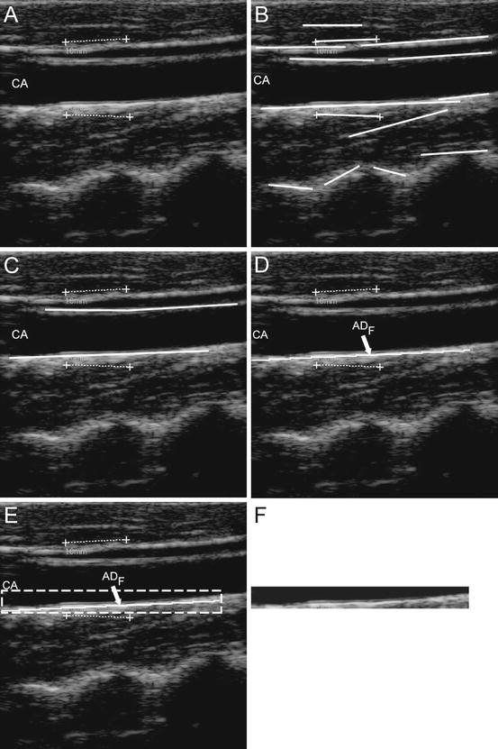
Fig. 17.4

Automated carotid identification (Stage-I) by CALEX 3.0. (a) Original cropped image. (b) Line segments. (c) Line segments corresponding to the near and far adventitia layers obtained through validation and classification [25]. (d) Final profile of the far adventitia (AD_F). (e) Determination of a Guidance Zone in which segmentation is performed (white dashed line). (f) Extracted Guidance Zone of the distal wall

The AD_F profile was used to derive a Guidance Zone (GZ) used by the subsequent Stage-II. This GZ must comprise the entire far wall along the carotid artery. Since the nominal IMT value is lower than 1 mm, it means that the distance between intima and media is about 13 pixels (since the pixel density of these images is 12.7 pixel/mm). Therefore, our GZ had the same horizontal width of the AD_F profile, and height equal to 30 pixels, which means about twice the size of the IMT. With this value, our GZ always comprised the distal (far) wall and a portion of the carotid lumen. The pixels in the GZ were then processed by Stage-II. Figure 17.4e shows the Guidance Zone automatically detected (white dashed rectangle), and Fig. 17.4f the cropped Guidance Zone containing the distal carotid wall.

3.2 Stage-II: Fuzzy-Based LI-MA Segmentation Strategy

The automated delineation or segmentation of the far wall is performed by relying on a fuzzy K-means classifier. The GZ was processed column-wise. The intensity profile of each column was fed as input to the fuzzy K-means classifier. Basically, we modeled the intensity profile as a mixture of three clusters of pixels: (1) the pixels belonging to the lumen, which have a low intensity; (2) the pixels belonging to the intima and media layers, which are characterized by an intermediate gray intensity; and (3) the pixels belonging to the far adventitia, which are bright and with high associated values. Therefore, we forced the number of clusters of our K-means classifier equal to three. The pixel at the boundary between the first and the second class was then taken as marker of the LI interface; the pixels at the boundary between the second and the third class were taken as the marker of the MA interface. The final LI and MA boundaries were obtained by the sequence of the LI and MA marker points of every column of the GZ. Figure 17.5 shows three samples of CALEX 3.0 LI/MA profiles.

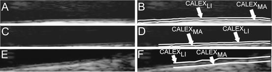
Fig. 17.5

Samples of CALEX 3.0 automated segmentation. The image is zoomed in the Guidance Zone

3.3 Stage-III: LI/MA Boundaries Refinement

Computer-generated boundaries might present local inaccuracies, caused by noise and image artifacts. Such inaccuracies are problematic in the framework of automated IMT measurement, because they can introduce a substantial error in the computer measurement of the IMT. Our CALEX 3.0 system is equipped with a third stage of post-processing that regularizes the LI/MA profiles and avoids inaccuracies. The two refinement strategies we introduced in CALEX 3.0 are lumen region detection and spike removal.

Lumen Region Detection via Pixels Classification

We introduced a lumen detection step to prevent the computer-generated profiles crossing or penetrating into the lumen region. Particularly, we observed that when the carotid lumen was characterized by a high degree of blood backscattering, the LI profile could become inaccurate and protrude or bleed into the carotid lumen. This error condition is caused by the incorrect pixel classification by Stage-II. The pixels belonging to the lumen can be easily detected by relying on the bidimensional distribution of the intensities and standard deviations. Specifically, we computed the average intensity and the standard deviation of the intensity values of the 10 × 10 square neighborhood of each pixel. We found that lumen points have a very low average intensity and a very low standard deviation, since they are almost black and surrounded by homogeneous dark pixels. Hence, by plotting a bidimensional histogram, we could mark all the pixels possibly belonging to the artery lumen. Figure 17.6 shows an example of lumen region detection on an image from our dataset.

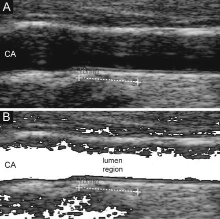
Fig. 17.6

Lumen region detection. (a) Original cropped image. (b) Lumen region detection. The pixels possibly belonging to the lumen are mapped to white

All the pixels possibly belonging to the artery lumen were marked according to the described procedure. Then, we forced the fuzzy K-means classifier of Stage-II to classify such lumen pixels into the first cluster. This avoided the LI profile bleeding into the artery lumen in 100% of the images.

Spike Detection and Removal

Small spikes can be present in the final LI/MA profiles. Again, such spikes can be generated by noise. Since the conversion factor of our database was 0.0787 mm/pixel, an IMT of 1 mm was be equivalent to 12.7 pixels. Therefore, we defined spike as a jump higher than six pixels in the LI/MA profiles, which means about half the nominal IMT value. All the spikes were detected and substituted by the average value of the 10 points neighboring the spiky point (5 points to the left and 5 to the right).

4 IMT Measurement and Performance Metric

The segmentation errors were computed by comparing automated tracings by CALEX 3.0 with manual segmentations, which were traced by expert sonographers by using a custom-made research prototype available system (ImgTracer™, Global Biomedical Technologies, Inc., California, USA). We used the Polyline Distance measure (PDM) as performance metric. A detailed description of the PDM can be found in previous works [33]. The fundamental equations of the PDM metric are reported in Appendices 1–3. Consider that the output of the CALEX 3.0 system consists of two profiles: LI and MA. Both the profiles consist of a certain number of vertices or points on the LI/MA borders. First, we compute the average distance of the vertices of LI with respect to the segments of MA and we call this value as D _LI-MA. Then, we compute the average distance between the vertices of MA with respect to the segments of LI and call such distance as D _MA-LI. The PDM is defined as the sum of D _LI-MA with D _MA-LI divided by the total number of vertices of the two profiles. The main advantage of using the PDM as performance metric is that it is almost insensible to the number of points constituting a profile.

For each image, we compared the IMT measured by CALEX 3.0 with the IMT value calculated from manual delineations (GT). We then computed the IMT bias (i.e., the difference between CALEX 3.0 measurement and GT IMT), the IMT absolute value (i.e., the absolute difference between CALEX 3.0 measurement and GT IMT), and the IMT squared error (i.e., the squared absolute difference between CALEX 3.0 measurement and GT IMT). A detailed description of the error metrics is reported by Appendix 1. We also computed the Figure-of-Merit (FoM) for CALEX 3.0, which corresponds to the percent agreement between the computer-estimated IMT, and manually measured IMT values (mathematical details are reported in Appendix 3).

Only gold members can continue reading. Log In or Register to continue