Fig. 11.1
An example of the result of statistical analysis of SPECT image. It is not easy to point out the hypoperfusion regions with visual inspection of SPECT image except for hypoperfusion in medial temporal regions. However, statistical analysis with easy z-score imaging software (eZIS) reveals hypoperfusion in precuneus in addition to hippocampal hypoperfusion. These results are quite persuasive and easy to understand for not only medical staffs but also patients and their families
11.3.1 Preprocessing (Normalizing and Smoothing)
Each individual has a different size and shape of the brain. In order to compare data from several subjects, all the images need to be in the same space. In eZIS which employs SPM, this is accomplished by “normalizing” the images into the space defined by the Montreal Neurological Institute (MNI) template. The detail of normalizing process is described by Ashburner, one of the developers of SPM [6].
Following spatial normalization, the image data would be “smoothed” or blurred. By smoothing, the signal-to-noise ratio is increased. It also ensures that the residual differences are closer to Gaussian and decreases the intersubject registration error. Another reason for smoothing is simplifying the ensuing results, producing fewer regions of significant difference to report [7]. The outline of preprocessing is illustrated in Fig. 11.2.
Fig. 11.2
A scheme of preprocessing. In order to compare data from several subjects, data are normalized to the space defined by the Montreal Neurological Institute template. Following spatial normalization, the image data are smoothed to be suited for statistical analysis
11.3.2 Generating Z-Score Images
After preprocessing, intensity of each image is normalized. Note that eZIS takes a different approach from SPM. In SPM, intensity normalization takes a two-step procedure. First, it calculates mean of an image. This averages all of the voxel values (VV) even outside the brain, so we need to threshold the image with certain value. Threshold is calculated by mean divided by 8. Then it calculates global value by averaging the VV above the threshold. Finally global value is set to 50 mL/min/100 g and each VV is adjusted with proportional scaling.
On the other hand, eZIS takes a straightforward procedure. First it applies a brain mask to preprocessed images. Then mean value is calculated with the masked images. Setting global value and adjusting VV is the same as SPM. Figure 11.3 illustrates how mean and VV of a certain voxel will change throughout the procedure. VV of a voxel coordinate [40 30 40] in the preprocessed image is 796.0 and mean VV is 368.8. Note that at this point, mean includes voxels outside the brain. After masking, VV at [40 30 40] remains the same, but the mean changes from 368.8 to 635.1. Now using proportional scaling eZIS sets mean as 50, VV at [40 30 40] will be  Understanding this procedure is important because sometimes we see apparent hyperperfusion regions in eZIS results. For example, global cerebral blood flow (CBF) of advanced demented patients is generally low such as 30 mL/min/100 g, but the regional CBF in primary sensory motor region is intact such as 45 mL/min/100 g. In this case, after intensity normalization, the adjusted regional CBF in primary somatosensory regions will be
  which will result in remarkable hyperperfusion in this region. In order to prevent misinterpreting the results, it is recommended to check the global CBF regularly.

Understanding this procedure is important because sometimes we see apparent hyperperfusion regions in eZIS results. For example, global cerebral blood flow (CBF) of advanced demented patients is generally low such as 30 mL/min/100 g, but the regional CBF in primary sensory motor region is intact such as 45 mL/min/100 g. In this case, after intensity normalization, the adjusted regional CBF in primary somatosensory regions will be which will result in remarkable hyperperfusion in this region. In order to prevent misinterpreting the results, it is recommended to check the global CBF regularly.Fig. 11.3
Illustration of how mean and voxel values (VV) of a certain voxel will change by masking and proportional scaling
Following intensity normalization, z-score at each voxel is calculated with the following equation.

Here SD stands for standard deviation. This equation can be rephrased like the following.

So if Z-score is 2, one can say that subject’s VV in a certain voxel is 2 standard deviation below average of control subjects. This equation also tells us that we need to prepare the mean and standard deviation of control subjects beforehand. Z-score highly depends on the quality of control subjects, so we need to keep in mind that using different control subjects might result in quite a different result.
11.4 SPECT Findings in Alzheimer’s Disease
SPECT findings of typical AD are characterized by hypoperfusion in (1) the parietotemporal association cortex, (2) posterior cingulate gyrus and precuneus; and (3) medial temporal areas [8]. It is also noteworthy that CBF of primary sensorimotor region is spared until the advanced stage. The yellow arrows in Fig. 11.4 point the characteristic hypoperfusion regions in AD and red arrow points the primary sensorimotor region where CBF is spared.
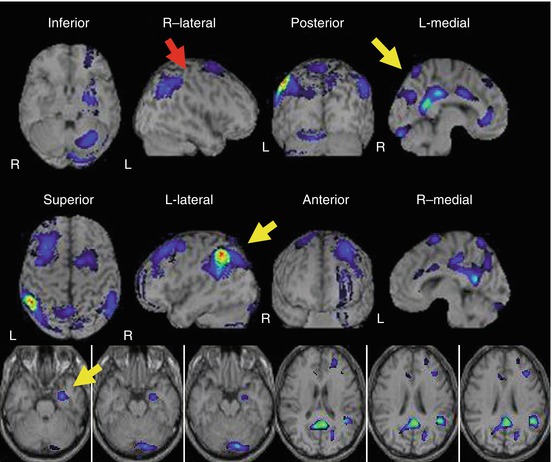
Fig. 11.4


SPECT findings of typical AD are characterized by hypoperfusion in the (1) parietotemporal association cortex, (2) posterior cingulate gyrus and precuneus, and (3) medial temporal areas. Note that CBF of the primary sensorimotor region is spared until the advanced stage. The yellow arrows point the characteristic hypoperfusion regions in AD, and the red arrow points the primary sensorimotor region where CBF is spared
Related posts:

Stay updated, free articles. Join our Telegram channel
Full access? Get Clinical Tree
