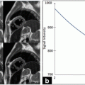
Carotid Artery Recognition System(CARS): A Comparison of Three Automated Paradigms for Ultrasound Images

Fig. 18.1

Automated cropping of the ultrasound DICOM image. The original image frame (left) is cropped (right). The white circle indicates the scanning depth, which could be used for manual computation of the calibration factor

2.1 CARSgd: Far Adventitia Border Detection Based on First-Order Derivative Gaussian Edge Analysis

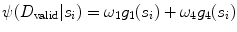
The completely automated technique we developed and named CARSdg consists of a novel and low-complexity procedure. Figure 18.2 shows the steps of the automatic CA recognition, starting with the automatically cropped image (Fig. 18.2aa), which constitutes the input to the recognition procedure. This is discussed in more detail here:

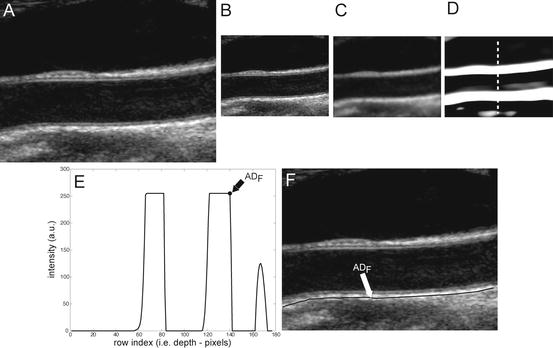
Fig. 18.2

CARSgd procedure for AD_F tracing. (a) Original cropped image. (b) Downsampled image. (c) Despeckled image. (d) Image after convolution with first-order Gaussian derivative (σ = 8). (e) Intensity profile of the column indicated by the vertical dashed line in panel d (AD_F indicates the position of the far adventitia wall). (f) Cropped image with far adventitia profile overlaid

Step 1: Fine to coarse downsampling. The image was first downsampled by a factor of two (i.e., the number of rows and columns of the image was halved) (Fig. 18.2bb). We implemented the downsampling method discussed by Zhen et al. [22], adopting a bi-cubic interpolation. This method was tested on ultrasound images and showed a good accuracy and a low computational cost [22]. Downsampling prepares the vessel wall’s edge boundary such that the vessel wall thickness tends to be equivalent to the scale of the Gaussian kernels (used in Step 3 for wall recognition). This paradigm will yield an automated recognition of the distal (far) adventitia layer. Thus a guidance zone can be built around this far adventitia border for wall segmentation. Fan et al. [23] adopted a similar approach to measure the diameter of the brachial artery. They used a Gaussian higher order filtering to create a guidance zone. Segmentation was then performed by relying on a template matching strategy.
Step 2: Speckle reduction. Speckle was attenuated by using a first-order local statistics filter (named as lsmv by the authors [24, 25]), which gave the best performance in the specific case of carotid imaging. This filter is defined by the following equation:

${J_{x,y }}=\bar{I}+{k_{x,y }}({I_{x,y }}-\bar{I})$

(18.1)
where I _x,yis the intensity of the noisy pixel, $\bar{I}$ is the mean intensity of a N × M pixel neighborhood, and k _x,yis a local statistic measure. The speckle-free central pixel in the moving window is indicated by J _x,y. Loizou et al. [24] mathematically defined ${k_{x,y }}=\frac{{\sigma_I^2}}{{{{\bar{I}}^2}\sigma_I^2+\sigma_n^2}}$ , where $\sigma_I^2$ represents the variance of the pixels in the neighborhood, and $\sigma_n^2$ is the variance of the noise in the cropped image. An optimal neighborhood size was shown to be 7 × 7. Figure 18.2cc shows the despeckled image. Note that the despeckle filter is useful in removing the spurious peaks if any during the distal (far) adventitia identification in subsequent steps.
Step 3: First-order derivative Gaussian edge (FODGE) operator. The despeckled image was filtered by using a 35 × 35 pixels first-order derivative of a Gaussian kernel. Figure 18.2dd shows the results of the filtering by the Gaussian derivative. The scale parameter of the Gaussian derivative kernel was taken equal to 8 pixels, i.e., half the expected dimension of the IMT value in an original fine resolution image. In fact, an average IMT value of say 1 mm corresponds to about 16 pixels in the original image scale and, consequently, to 8 pixels in the coarse or downsampled image. The white horizontal stripes of Fig. 18.2dd are relative to the proximal (near) and distal (far) adventitia layers.
Step 4: Automated far adventitia (AD_F) tracing. Figure 18.2ee shows the intensity profile of one column of the filtered image of Fig. 18.2dd. The proximal and distal walls are visible as intensity maxima saturated to the value of 255. To automatically trace the profile of the distal wall, we used a heuristic search applied to the intensity profile of each column. Starting from the bottom of the image, we search for the first white region consisting of width of at least 6 pixels (computed empirically). The deepest point of this region (i.e., the pixel with the higher row index) marked the position of the far adventitia (AD_F) layer on that column. The sequence of the points resulting from the heuristic search for all the image columns constituted the overall automated AD_F tracing.
Step 5: Upsampling of far adventitia (AD_F) boundary locator. The AD_F profile was then upsampled to the original fine scale and superimposed over the original cropped image (Fig. 18.2ff) for both visualization and performance evaluation.

This Stage-I essentially consists of an architecture combining fine-to-coarse downsampling for wall scale reduction, despeckle filtering, first-order derivative Gaussian Kernel edge (FODGE) filtering for wall extraction, and Heuristic-based peak detection for final segmentation of the far adventitia borders. The matching between the downsampled wall thickness and the Gaussian Kernel size (scale) ensured optimal representation of the artery. If the FODGE kernel size did not match the theoretical IMT of 8 pixels, the overall CARSgd performance decreased from 100% $(\sigma =8)$ to 94% for $\sigma =6$ and 97% for $\sigma =10$ . We chose to downsample the image and match the wall size to the FODGE kernel and not vice versa to avoid higher error propagation and to reduce the computational burden.

2.2 CARSia: Far Adventitia Border Detection Using Feature Extraction and Fitting

CARSia exploits the image information in order to automatically detect far adventitia [16]. This is based on the assumption that there exists a dark, low-intensity region (the lumen region) between the two bright, higher intensity regions (the near and far wall adventitia layers). Thus, the basic idea of CARSia is to exploit the geometrical and intensity features of the carotid artery representation to recognize the artery walls. The first step is the definition of “seed points.” A seed point is a local intensity maxima located on the CA wall. Seed points are clustered from the other intensity maxima by a linear discriminator (which we preliminary trained on a subset of 15 images [16]). Once detected, seed points are then linked to form line segments. An intelligent procedure is applied to remove short or false line segments by computing the validation probability $P({D_{\mathrm{valid}}}|{s_i})$ [see (18.2) and (18.3)] and join close and aligned segments by computing the connectability probability $P({D_{\mathrm{conn}}}|{s_i})$ [see (18.4) and (18.5)]. This procedure avoids over-segmentation of the artery wall. Therefore, line segments classification extracts the line pair that contains the artery lumen in between.

$P({D_{\mathrm{valid}}}|{s_i})=\exp \left\{ {-\psi ({D_{\mathrm{valid}}}|{s_i})} \right\}$

(18.2)

where the energy function $\psi (\cdot )$ is based on the support ${g_1}({s_i})$ and the width stability ${g_4}({s_i})$ and is defined according to the following formula:

$\psi ({D_{\mathrm{valid}}}|{s_i})={\omega_1}{g_1}({s_i})+{\omega_4}{g_4}({s_i})$

(18.3)

$P({D_{\mathrm{conn}}}|{s_i},{s_j})=\exp \{-\psi ({D_{\mathrm{conn}}}|{s_i},{s_j})\}$

(18.4)

where the energy function $\psi (\cdot )$ is based on proximity ${h_1}({s_i},{s_j})$ and alignment ${h_2}({s_i},{s_j})$ :

$\psi ({D_{\mathrm{conn}}}|{s_i},{s_j})={{\omega^{\prime}}_1}{h_1}({s_i},{s_j})+{{\omega^{\prime}}_2}{h_2}({s_i},{s_j})$

(18.5)

Here, ω ₁, ω ₄, ${{\omega^{\prime}}_1}$ , and ${{\omega^{\prime}}_2}$ are weights determined by the training data. For each line segment ${s_i}$ we defined four features:

(a)

Support, defined as the number of seed points contained by the segment ${s_i}$ (indicated by ${g_1}({s_i})$ )

(b)

Residue, defined as the mean squared error of the seed points with respect to their perpendicular distance from ${s_i}$ (indicated by ${g_2}({s_i})$ )

(c)

Spread, defined as the shortest path length connecting the seed points divided by the number of seed points ${s_i}$ contains (indicated by ${g_3}({s_i})$ )

(d)

Width stability, defined as the percentage of points along the fitted line segments ${s_i}$ whose width (perpendicular distance to the nearest intensity edge) is within some tolerance of the estimated width of the adventitial layers (indicated by ${g_4}({s_i})$ )

These are computed as follows: ${g_1}({s_i})$ is mathematically defined and computed as the number of seed points present on the line segment ${s_i}$ .

${g_2}\left( {{s_i}} \right)$ is the residue and is computed as the average Euclidean distance from the seed points to the line segment ${s_i}$ . Thus it is the perpendicular distance from the seed point to the line segment ${s_i}$ .

${g_3}({s_i})$ is the spread function defined as the shortest path length connecting the seed points divided by the number of seed points ${s_i}$ contains.

We compute the length of s _ias follows: (a) selection of any two seed points that s _icontains, and then, calculate the Euclidean distance; (b) the maximum Euclidean distance is the length of ${s_i}$ .

${g_4}({s_i})$ is mathematically defined as the percentage of points along the fitted line segments ${s_i}$ whose width (perpendicular distance to the nearest intensity edge) is within some tolerance of the estimated width of the adventitial layers. The algorithmic steps for computation of ${g_4}({s_i})$ are as follows:

Application of the Canny edge detector on the original image. Canny edge detector uses a multistage algorithm to detect a wide range of edges in images. Because it is susceptible to noise present on raw unprocessed image data, we thus convolve the raw image with an optimal Gaussian filter.

For each line segment, find its closest edge. This can be done by applying connected component analysis to the binary Canny edges. Then calculate the distance from a line segment to an edge and then sort the distance values.

For each seed point on a line segment, we calculate the distance d _ito the closest edge.

We then compute the average distance R as the average radius of this line segment s. To remove the outliers caused by the background noise we calculate the threshold, which is the ratio r _i = d _i/R. Our lower threshold bound is 0.8 and upper threshold bound is 1.25. Setting these threshold values can effectively remove most of outliers.

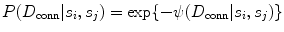
Finally, calculate the percentage of seed points that meet the criteria above which is called the width stability [16, 17].

Details about the definition of the above parameters are described in our previous paper [16]. Figure 18.3 summarizes CARSia functioning.

Fig. 18.3

CARSia (integrated approach) recognition strategy. (a) Original image. (b) Automatically identified line segments (black lines). (c) Final AD_F tracing after line segments validation and combination

2.3 CARSsa: Local Statistics Approach

The automated approach based on local statistics was one of the first we developed and was the basis of many studies we conducted [14, 15, 17, 26–32].

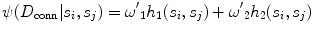
This approach is based on the assumption that carotid representation can be thought of as a mixture model with varying intensity distributions. This is because the (a) pixels belonging to the vessel lumen are characterized by low mean intensity and low standard deviation; (b) pixels belonging to the adventitia layer of the carotid wall are characterized by high mean intensity and low standard deviation; and (c) all remaining pixels should have high mean intensity and high standard deviation. As a result, we derived a bi-dimensional histogram (2DH) of the carotid image. For each pixel, we considered a 10 × 10 neighborhood of which we calculated the mean value and the standard deviation. The mean values and the standard deviations were normalized to 0 and 1 and were grouped into 50 classes each having an interval of 0.02. The 2DH was then a joint representation of the mean value and standard deviation of each pixel neighborhood. In previous studies, we showed that pixels belonging to the lumen of the artery are usually classified into the first classes of this 2DH [9]: expert sonographer manually traced the boundaries of the CA lumen and observed the distribution of the lumen pixels on the 2DH. Overall results revealed that pixels of the lumen have a mean values classified in the first four classes and a standard deviation in the first seven classes. We therefore consider a pixel as possibly belonging to the carotid lumen if its neighborhood intensity is lower than 0.08 and if its neighborhood standard deviation is lower than 0.14. Figure 18.4 shows the lumen region selection process in four images: Fig. 18.4aa depicts the original image after automatic cropping; Fig. 18.4bb depicts the 2D histogram (2DH) showing the relationship between the normalized mean and normalized standard deviation. The gray region in the 2DH represents what we consider the lumen region of the carotid artery. All the image pixels falling into this region have been depicted in gray in Fig. 18.4cc. This example shows how the local statistic is effective in detecting image pixels that can be considered as belonging to the CA lumen.

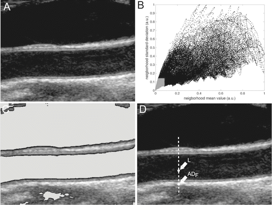
Fig. 18.4

CARSsa (signal processing) strategy for far wall adventitial tracing. (a) Original image. (b) Bidimensional histogram (2DH). The gray portion of the 2DH denotes the region in which we suppose to find only lumen pixels. (c) Original image with lumen pixels overlaid in gray. (d) Sample processing of one column, with the marker points of the far (AD_F) adventitia layer and of the lumen (L)

To avoid incorrect detection of our ADF, we had to attenuate the superimposed noise and random intensity peaks. We therefore used the low-pass filter (Gaussian Kernel Size 29 × 29, with $\sigma =1$ ) and convolved it with the image to lessen the noise and speckle effect. Schematically, the following are the steps for processing the intensity profile:

(i)

AD _Ftracing: the procedure started from the bottom most point and searched for the first maxima with an intensity value above the 90th percentile of the intensity distribution along that profile. This point was marked as possible far adventitia (AD_F) candidate. Starting from the bottom most point and searching for a local intensity maximum yielded the AD_F candidate selection quite robust, due to the hyperechoic appearance of the adventitia layer. The strong low-pass filtering preliminary to this choice attenuated possible high-intensity noisy points located above the adventitia layer.

(ii)

Lumen tracing: For lumen estimation point, the algorithm moved upwards along the row (decreasing row value) and searched for a pixel (point) possibly belonging to the lumen. The lumen candidate was the first minima point whose neighborhood mean intensity and standard deviation values matched the criteria of the 2DH (i.e., normalized mean value lower than 0.08 and normalized standard deviation lower than 0.14, respectively).

When the two candidate points along the column were found, they were plotted on the original image in correspondence of their row index (and of the column index under analysis). If the row index reached 1 (or the last row) before the two points were found, the column was discarded and marked as unsuitable to segmentation. Figure 18.4dd shows the marked points on a sample image column.

3 Image Database and Preprocessing Steps

We describe here the image dataset we used for performance analysis and validation of CARS.

Our database consisted of 365 B-model images collected from four different institutions/hospitals around the world. They are as follows:

The Neurology Division of the Gradenigo Hospital of Torino (Italy), which provided 200 images.
The Cyprus Institute of Neurology of Nicosia (Cyprus), which provided 100 images.
The Hospital de S. João do Porto (Portugal), which provided 23 images [33, 34].
The Department of Radiology of the University Hospital of Cagliari (Italy), which provided 42 images.

The complete description of the image database and of the patient’s demographics is reported by Table 18.1. All the Institutions took care of obtaining written informed consent from the patients prior to enrolling them in the study. The experimental protocol and data acquisition procedure were approved by the respective local Ethical Committees.

Table 18.1

Image database and patient demographics

Institution	Total images (N)	Conversion factor ( $\tau$ ) (mm/pixel)	Ultrasound scanner	Patients	Age
Torino (Italy)	200	${\tau_{\mathrm{Torino}}}=0.0625$	ATL HDI5000	150	69 ± 16 years (50–83 years)
Nicosia (Cyprus)	100	${\tau_{\mathrm{Nicosia}}}=0.0600$	ATL HDI3000	100	54 ± 24 years (25–95 years)
Porto (Portugal)	23	${\tau_{\mathrm{Porto}}}=0.0900$	ATL HDI5000	23 Only gold members can continue reading. Log In or Register to continue Share this: Click to share on Twitter (Opens in new window) Click to share on Facebook (Opens in new window) Related posts: Relationship Between Plaque Echogenicity and Atherosclerosis Biomarkers Quantitative Magnetic Resonance Analysis in the Assessment of Cardiac Diseases Quantitative Computed Tomography Analysis in the Assessment of Coronary Artery Disease Visualization of Atherosclerotic Coronary Plaque by Using Optical Coherence Tomography Hypothesis Validation of Far Wall Brightness in Carotid Artery Ultrasound for Feature-Based IMT Measurement Using a Combination of Level Set Segmentation and Registration Segmentation of Carotid Ultrasound Images Stay updated, free articles. Join our Telegram channel Tags: Multi-Modality Atherosclerosis Imaging and Diagnosis Aug 24, 2016 \| Posted by admin in GENERAL RADIOLOGY \| Comments Off on Carotid Artery Recognition System(CARS): A Comparison of Three Automated Paradigms for Ultrasound Images Full access? Get Clinical Tree Get Clinical Tree app for offline access Get Clinical Tree app for offline access