Fig. 8.1
General procedure of 3D plaque geometry reconstruction
Fig. 8.2
Segmentation results for the symptomatic patients superimposed on T2-weighted MRI images (a) and reconstructed 3D plaque geometry (b)
2.3 Plaque Stress Analysis by FSI Simulation
The carotid arterial wall was assumed to be nonlinear, isotropic, and incompressible. The 3D nonlinear Mooney–Rivlin model in ANSYS11.0 was used to describe the material property, the strain energy density function W was
where I 1 and I 2 are the first and second strain invariants, d is the material incompressible parameter, J stands for the ratio of the deformed volume over the un-deformed volume of materials, C 10, C 01, C 20, C 11, and C 02 are material constants. In the study, C 10 = 50.445 kPa, C 01 = 30.491 kPa, C 20 = 40 kPa, C 11 = 120 kPa, C 02 = 10 kPa, and d = 1.44e−7, derived from existed literatures [29]. Lipid core was much softer with 2 kPa for the Young’s modulus and 0.49 for Poisson ratio. The structure model was meshed with an unstructured mesh consisting of nearly 90,000 10-node 3D tetra elements. The computational nodes at the efferent planes of ICA and ECA were fixed in all directions and an axial pre-stretch of 11% (based on the shunk procedure in plaque geometry reconstruction).
(8.1)
The fluid domain was meshed in ICEM CFD11.0 with a much finer grid of around 1,000,000 3D tetra cells. Blood was treated as an incompressible, Newtonian fluid with a viscosity of 4 × 10⁻³ Pa s and a density of 1,067 kg m−3. The flow was assumed to be laminar. Transient simulations were carried out with time-dependent pressure at the inlet of the CCA and mass flow rates at the ICA and ECA. In this study, the boundary conditions for the two subjects were assumed to be the same as in Fig. 8.3. The fully coupled FSI simulation details also can be found in ref. [10].
Fig. 8.3
Mass flow rates for ICA and ECA (a) and pressure profile at CCA (b)
2.4 Stress Analysis Results
The first principle stress (FPS) was used to represent the plaque wall tensile stress, the strongest stretching stress. Figure 8.4 shows the stress distributions between the symptomatic (column 1) and asymptomatic (column 2) patients. Figure 8.4a1, b1 shows the FPS distribution in the whole plaque with longitudinal cutting view. Generally FPS is higher at the luminal wall, lower at the outer arterial wall, and lowest in the lipid region. The local high stress concentrations could be identified in the plaque region at both patients, indicated by arrows in Fig. 8.4a1, b1. The maximum FPS value is much higher in the symptomatic patient (227.7 kPa) than the asymptomatic patient (134.9 kPa). Figure 8.4a2, b2 presents FPS distributions in the transversal planes covering the whole plaque region. For the sections with a thin fibrous cap, the stress concentration regions appear at one or both edges of the lipid core (or plaque shoulders).
Fig. 8.4
FPS distributions for one symptomatic patient (a) and one asymptomatic patient (b)
Stress distribution in the fibrous cap has been considered to be closely related to plaque rupture. The fibrous cap surface in the lumen side was extracted, covering the lipid core, to clearly show the stress distribution in the plaque region. The fibrous cap thickness (FCT), defined as the shortest distance between the fibrous cap surface (lumen side) and lipid region, is shown in Fig. 8.5a1, b1. Although MR image spatial resolution is 0.39 mm, the 3D surface interpolation during model reconstruction can still produce fibrous cap regions with a thickness less than 0.39 mm. The minimum FCT in the symptomatic subject is much smaller than the asymptomatic subjects (0.087 mm vs. 0.177 mm). Figure 8.5a2, b2 shows corresponding FPS distributions in fibrous cap surfaces. Generally, the high stress regions are well correlated with the thin fibrous cap regions; especially for the asymptomatic patient, the high stress region upstream is corresponding to a very thin fibrous cap location. While in symptomatic patient, the highest stress region does not locate in the thinnest fibrous cap region (downstream plaque); this may be resulted in part from the blood pressure drop at downstream plaque. Linear correlation analysis of the FPS and FCT was performed for the two plaques by comparing the FPS and FCT value at every computational node on the fibrous cap surface in the lumen side. Figure 8.6a, b presents the scatter plot between FCT and FPS. The correlation results were r = −0.434 with p < 0.05 for the symptomatic patient and r = −0.692 with p < 0.05 for the asymptomatic patient.
Fig. 8.5
FCT and FPS distributions for symptomatic (a) and asymptomatic (b) patients
Fig. 8.6
Scatter plots of fibrous cap thickness and plaque wall stress for the symptomatic (a) and asymptomatic patients (b)
3 Patient-Specific Material Model Based on In Vivo MRI
Recent studies have demonstrated that it is possible to obtain patient-specific material model from in vivo human data [22], which enable plaque stress analysis to be much closer to the real situation rather than a general material model from existed literatures or obtained by ex vivo experiments. Therefore in this part, the method proposed by Masson [22] was used to determine arterial properties from in vivo data and applied the material properties to plaque stress analysis for one subject. An idealized 3D arterial wall section representing CCA was constructed based on in vivo MR images. Phase contrast MR images, residual stress, perivascular stress, and fiber-reinforced, hyperelastic effect of arterial tissue were included in the mechanical model. The fitted material parameters were applied to a real plaque stress analysis. It is believed that the procedure of using patient-specific material model will yield more realistic plaque stresses.
3.1 MRI Data Acquisitions
The MRI acquisition protocol was the same as in Sect. 2. Phase contrast MR images at common carotid artery were obtained to provide the luminal area change over one cardiac cycle as in Fig. 8.7a; the bright region, indicated by the arrow, is the lumen region; however there is little information regarding arterial wall. Figure 8.7b shows the luminal radius change of the CCA section over one cardiac cycle. Due of lack of pressure information, a pressure profile (denoted as measured pressure) was chosen as in Fig 8.3b by rescaling the pressure range of 80–110 mmHg according to luminal area change over time at CCA.
Fig. 8.7
In vivo data in CCA. (a) Phase contrast MRI of a CCA section; (b) luminal radius change
3.2 Kinematics of Idealized Arterial Wall
CCA section in Fig. 8.7a was considered to be a thick-walled circular cylinder in order to theoretically calculate stretch ratio in radial and circumferential directions by using a cylindrical coordinate system, that is, (e r , e θ , e z ). Therefore the deformation field of the CCA section over one cardiac cycle could be calculated from two successive motions [17]. Three configurations were considered as  : stress free and excised configuration
  ;
;  : intact and unloaded configuration (ρ, ϕ, ξ);
  : in vivo loaded configuration (r, θ, z). The three configurations can be found in Fig. 8.8.
: stress free and excised configuration ; : intact and unloaded configuration (ρ, ϕ, ξ); : in vivo loaded configuration (r, θ, z). The three configurations can be found in Fig. 8.8.Fig. 8.8
Three different configurations of the intact CCA from stress free to load free and loaded state
If a material particle is considered in the arterial wall, such as the particle indicated by ‘ ’ in Fig. 8.8, then
  ,
,  , x(r, θ, z) are the configurations of
  ,
,  , and
, and  , respectively. By employing the relations from Humphrey [17],
where t is the time, Θ 0 is the open angle when arterial wall is excised. Λ is the axial stretch accounting for axial residual stress from  to
to  . λ is the in vivo load-induced axial stretch, which is assumed to be constant over cardiac cycles. R i and r i are the inner radiuses in
  and
and  ; R m and r m are the radiuses at the medial–adventitial interface.
’ in Fig. 8.8, then , , x(r, θ, z) are the configurations of , , and , respectively. By employing the relations from Humphrey [17],(8.2)
(8.3)
to . λ is the in vivo load-induced axial stretch, which is assumed to be constant over cardiac cycles. R i and r i are the inner radiuses in and ; R m and r m are the radiuses at the medial–adventitial interface.The deformation gradient tensor from  to
to  can be defined as
  , that is
![$$ F=\left[ {\begin{array}{*{20}{c}} {\frac{{\partial r}}{{\partial R}}} & {} & {} \\ {} & {\frac{{\pi r}}{{{\Theta_0}R}}} & {} \\ {} & {} & {\lambda \Lambda } \\ \end{array}} \right]=\left[ {\begin{array}{*{20}{c}} {{\lambda_r}} & {} & {} \\ {} & {{\lambda_{\theta }}} & {} \\ {} & {} & {{\lambda_z}} \\ \end{array}} \right] $$](/wp-content/uploads/2016/08/A271459_1_En_8_Chapter_Equ00084.gif)
where λ r , λ θ , and λ z are principle stretch ratios in radial, circumferential, and axial directions. The left and right Cauchy–Green tensors are
to can be defined as , that is(8.4)
(8.5)
The local volume ratio is
(8.6)
Generally arterial wall is considered to be impressible, therefore J = 1. Then by applying (8.2)–(8.6) with J = 1,
(8.7)
Integrating from r i and R i to r and R respectively,
(8.8)
Therefore the stretch ratio in radial direction is
(8.9)
3.3 Constitutive Modeling of Arterial Wall
The mechanical response of the CCA section is considered to be anisotropic hyperelastic. Because the material properties in adventitial layer is different from medial layer, and different collagen fiber configurations compared to medial layer, in order to simplify the solution procedure, as in Masson’s study [22], only medial and intimal layers were studied in this study. The strain energy function proposed by Gasser [14] was used to model the CCA section with two families of collagen fibers embedded in a soft incompressible ground matrix, which is also available in Abaqus 6.8. The associated strain energy function W is
(8.10)
(8.11)
a, D, k 1, and k 2 are material parameters. κ denotes the level of dispersion in the fiber directions, in this study κ = 0, which means fibers from one family are perfectly aligned along one direction. f represents one fiber family, N is the total number of fiber families. Two families of fibers (f 1, f 2) are considered in this study (N = 2), and the fibers only distribute in circumferential and axial directions, no fiber in radial direction, as shown in Fig. 8.9. The angles of f 1 and f 2 with circumferential direction are  and
and  . In this study,
  is equal to
  .
.
 Relationship Between Plaque Echogenicity and Atherosclerosis Biomarkers
 Quantitative Magnetic Resonance Analysis in the Assessment of Cardiac Diseases
 Quantitative Computed Tomography Analysis in the Assessment of Coronary Artery Disease
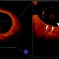 Visualization of Atherosclerotic Coronary Plaque by Using Optical Coherence Tomography
 Hypothesis Validation of Far Wall Brightness in Carotid Artery Ultrasound for Feature-Based IMT Measurement Using a Combination of Level Set Segmentation and Registration
 Segmentation of Carotid Ultrasound Images


and . In this study, is equal to .Related posts:
Relationship Between Plaque Echogenicity and Atherosclerosis Biomarkers
Quantitative Magnetic Resonance Analysis in the Assessment of Cardiac Diseases
Quantitative Computed Tomography Analysis in the Assessment of Coronary Artery Disease
Visualization of Atherosclerotic Coronary Plaque by Using Optical Coherence Tomography
Hypothesis Validation of Far Wall Brightness in Carotid Artery Ultrasound for Feature-Based IMT Measurement Using a Combination of Level Set Segmentation and Registration
Segmentation of Carotid Ultrasound Images
Stay updated, free articles. Join our Telegram channel
Full access? Get Clinical Tree
