Fig. 7.1
Decision tree scheme for checking and correcting of diffusion data. Std standard deviation, interslice inst. interslice instabilities, PIS physically implausible signal, MDC motion-distortion correction, TV total variation, FA/DEC direction-encoded FA map, perc. percentage
Recognition and Correction of Artifacts
Eddy Current-Induced Distortions
Origin
Conductive elements of the MRI scanner (e.g., the gradient coils) permit the flow of electric charges. When a conductor is located in a changing magnetic field, this will induce currents in the conductor. Because their flow patterns resemble swirling eddies in a river, they are called eddy currents. Besides gradients for spatial localization of the MR signal, additional magnetic gradients are used to make MR sensitive to diffusion. The diffusion-sensitizing gradients have to be switched on and off very rapidly, and induce eddy currents [2] in conductors present. The eddy currents , in turn, induce additional magnetic gradient fields which will change the actual diffusion gradient, as can be seen in Fig. 7.2b, where the actual diffusion gradient is different from the desired one in Fig. 7.2a. The effect on the DWIs is twofold: overlap of the changed diffusion gradient with spatial encoding gradients will lead to geometric distortions and thus misalignment of individual DWIs; and the deviation of the diffusion gradient from what we expect will lead to errors in diffusion estimates.
Fig. 7.2
Diffusion MR sequences. (a) For the standard, once-refocused, diffusion preparation, after the excitation (90° RF pulse) there are two gradients that sensitize the signal to diffusion, with a refocusing pulse (180° radio-frequency (RF) pulse) at half the echo time (TE/2) to form an echo during the readout. (b) The diffusion gradient is not as desired and overlaps with the spatial encoding gradients. (c) TRSE: The twice-refocused diffusion preparation (bottom line) has two refocusing pulses splitting four gradient blocks to form an echo during the readout
Recognition and Correction in Acquisition Stage
When eddy current-induced fields overlap with the spatial encoding period of the image acquisition, this will lead to geometric distortions. These distortions are visible in the raw DWIs in the phase-encoding direction (PE, most commonly anterior–posterior or y-direction) and depend on the direction of the eddy current gradient. An eddy current gradient in left–right (x) direction will result in a shear in the axial (xy) plane, assuming that the PE direction is anterior–posterior (y). Likewise, an eddy current gradient in y-direction causes scaling in y-direction (Fig. 7.3a shows compression in y-direction), whereas eddy current gradients in inferior–superior (z) direction translates each slice in y-direction dependent on the slice position [3].
Fig. 7.3
Example of DW image with scaling induced by eddy currents in the phase-encoded anterior–posterior (AP, indicated by the arrows) direction (a), compared to the undistorted B0 image (b). The lines overlaid in red indicate brain edges and boundaries of the undistorted B0 image. (c) Raw data in which the effect of eddy currents is minimized
Generation of eddy currents is inevitable in diffusion MRI; however, there are methods to minimize them. Replacing the single-refocused spin-echo diffusion preparation (Fig. 7.2a) by a twice-refocused spin-echo (TRSE) preparation (Fig. 7.2c) reduces the eddy currents resulting in less severe geometric distortions [4]. This is also called dual spin-echo (DSE) diffusion imaging . The TRSE/DSE diffusion sequence is available in most, if not all, recent MRI scanners, making this an easy to use option. Figure 7.3c shows a raw image with minimal eddy current distortions. The downside of a TRSE sequence is a small increase in echo time (TE), caused mainly by the additional 180 pulse. As a result, the signal-to-noise ratio (SNR) decreases and the repetition time (TR) may increase, which would result in a longer acquisition time.
Recognition and Correction in Image Processing Stage
Different geometric distortions of every individual DWI will result in misalignment of the images, which will, in general, affect diffusion-derived measures that are estimated on a voxel-by-voxel basis. Eddy current-induced misalignment artifacts become visible as bands of increased FA at the periphery of the brain (Fig. 7.4a) but, although less pronounced, are also present throughout the brain. The direction-encoded color (DEC) map s [5] furthermore show a dominant orientation in these bright rims, which is typical for eddy current-induced geometric distortions when they are only visible in the phase-encoding (PE) orientation of the image.
Fig. 7.4
(a) DEC map showing an orientational bias in the high anisotropy rim at the periphery of the brain. (b) The same map calculated after distortion correction
Correction for eddy current-induced distortions is commonly done in the diffusion MRI image processing pipeline. Various image registration based methods have been developed for correction [2, 6, 7]. Typically, mutual information is used to register all DWIs to the non-DW (b = 0) image, which has no eddy current-induced distortions. For this purpose no additional scans are needed. Figure 7.4b displays the DEC map after correction.
Besides image distortions, eddy currents can also influence diffusion measurements in another way. Figure 7.2b already showed that the actually applied diffusion gradient differs from the desired one. The diffusion weighting of an image is thus not exactly what we expect, which will result in errors in the estimates of the diffusion parameters. This is often hard to recognize and impractical to correct for.
Subject Motion
Origin
The acquisition of a typical clinical DTI dataset takes around 5–10 min, for research purposes this can even be longer. Although subjects are instructed to lie still during a scan, head or body motion is difficult to avoid. Motion can be subdivided into translations (in x-, y-, and z-direction) and rotations (yaw, pitch, and roll). Many DWIs have to be acquired to estimate diffusion properties accurately, and misalignment due to motion will lead to errors in these estimates.
Recognition and Correction in Acquisition Stage
Instead of a time-consuming detailed slice-by-slice inspection of the raw DW MRI data, subject motion can also be investigated by looping through the DW images at a frame rate of approximately ten frames per second, or quickly toggling between the first and last acquired DW MRI image.
During acquisition, all care should be taken to immobilize the subject. This is commonly done by placing cushions, or pads, between the subject’s head and the inside of the head coil. This makes it easier for the subject to keep his or her head still.
Even for the most willing and cooperative subjects, head motion is likely to occur to some extent. Slight movement of the brain may result in a mismatch between subsequent slices, which means these slices cannot be combined correctly. Several new pulse sequences have been proposed that can correct for in–plane motion, e.g., PROPELLER or SNAILS [8]. However, these cannot correct for through–plane motion . Prospective volume registration can account for through-plane motion. Here, the field-of-view (FOV) is repositioned after each 3D image volume, so after each TR. This method can correct the motion for any subsequent volume accurately, but the volume in which motion occurred is corrupt and must be re-acquired, elongating the scan time. To truly account for any motion, however, the motion must be detected with a higher temporal resolution. Zaitsev et al. [9] proposed such a real-time prospective motion correction setup: when head motion is detected, the imaging field-of-view is adjusted accordingly for the next excitation. Their system used a mouthpiece with markers outside the mouth that could be imaged by optical cameras outside of the magnet bore. In this way, rigid body motion of the head can be detected and corrected for a wide range of rotations and translations. Recent advances in this field were focused on ease-of-use as well as correction accuracy, with methods that use a small object attached to the subject’s forehead that is imaged by a camera within the bore, capable of correcting translations and rotations as small as 10 μm and 0.01° [10, 11]. For an extensive overview, one is referred to [12]. Currently, these methods are transforming from a purely developmental setup to products shared between neuroscientific research groups.
Recognition and Correction in Image Processing Stage
Subject motion will, just like eddy current geometric distortions, result in misregistration of DW volumes. This misregistration can in some cases also be recognized by rims of high anisotropy with orientational bias at the periphery of the brain, but this will, in contrast to misregistration produced by eddy currents, appear on all sides of the brain (Fig. 7.5a). In other cases, overall changes in FA or MD can be observed (Fig. 7.5b). In addition to DEC maps, misregistration artifacts (resulting from either eddy currents or subject motion) can also be recognized by inspecting images of the standard deviation across the DWIs, in which the size and brightness of the rims at brain edges and tissue interfaces reflect the degree of misalignment (Fig. 7.5c). Recognition and correction of subject motion on these maps is not always straightforward and depends largely on the kind of motion (abrupt or gentle, small or large).
Fig. 7.5
Subject motion can be recognized on FA/DEC maps by a bright rim (a) or an overall change of FA (b). (c) When plotting the standard deviation across all DWIs, bright rims at brain edges indicate misalignment. (d–f) show the same maps, corrected for subject motion
Image registration is commonly employed in diffusion MRI to correct for subject motion, and uses six parameters in total for translation and rotation. The corrected maps are visualized in Fig. 7.5d–f. The total transformation of eddy current distortion correction and subject motion are ideally applied at once on the original images [2]. A complication when dealing with registration of DWIs is that they contain directional information: diffusion gradients are applied in a specified direction. When the subject is rotated, one should rotate the b-matrix associated with each DWI. Neglecting to rotate the b-matrix can lead to incorrect diffusion metrics and erroneous tractography [13].
Interslice Instabilities
Origin
A specific type of motion artifact is interslice instability. This is discussed separately, since it only arises when motion occurs during an acquisition in which slices are scanned interleaved, i.e., even and odd-numbered slices of an EPI volume are collected sequentially (so first slices 1, 3, 5… and subsequently slices 2, 4, 6…).
Recognition and Correction in Acquisition Stage
Although it seems straightforward, checking the raw data in orthogonal views other than the slice direction is often omitted. Interslice instabilities such as intensity differences between slices resulting from interleaved acquisition can be recognized on these orthogonal views, see Fig. 7.6a. Artifacts arising from the interleaved acquisition are visible in the corpus callosum and at the brain edges, and result in signal dropouts. The best way to prevent these artifacts if they are motion related is to properly immobilize the subject or to use prospective motion correction as discussed above.
Fig. 7.6
(a) Interslice instabilities might not be visible on the axially interleaved acquisition plane, but becomes visible on the orthogonal planes in a DWI volume. (b) DEC map with interleave artifact
Recognition in Image Processing Stage
Interslice instabilities can become visible on FA DEC maps. The influence of motion in combination with interleaved acquisition is illustrated in Fig. 7.6b, where the artifact becomes apparent in different brain regions, such as the corpus callosum.
Table Vibrations
Origin
Table vibrations are the result of low-frequency mechanical resonances of the system due to application of the diffusion gradients [14, 15]. Spatial phase ramps in the phase image occur when neighboring voxels move over a different distance. These phase ramps correspond with shifts in k-space that result in signal loss. The amount of signal loss for a standard b-value of 1000 s/mm2 can be 5–17 %, and increases with the b-value. Moreover, the twice-refocused spin-echo sequence suffers more from these vibrations due to the even more rapid switching of the gradients [15]. So, although the TRSE sequence ameliorates the eddy current-induced distortions, one must ensure that it does not come at the cost of increased table vibration.
Recognition and Correction in Acquisition Stage
Table vibrations can result in localized signal loss, which is not a result of diffusion. The movement resulting from vibration is primarily directed in left–right direction, and the artifact is therefore visible in DWIs with a large component of the diffusion gradient in the left–right direction. Figure 7.7 illustrates this signal loss in a left–right sensitized image. When the region of signal loss overlaps with pathology, important diagnostic information can get lost.
Fig. 7.7
Signal dropouts in DWIs with a large component of the diffusion gradient in left–right orientation resulting from table vibrations
Most diffusion protocols do not acquire the whole k-space, but use partial coverage instead to shorten TE which reduces scan time and increases SNR. In case of partial k-space acquisitions, vibrations could move the center of k-space out of the scanned k-space, resulting in severe loss of information for proper reconstruction of the DWI. Several acquisition options exist to reduce vibrations. Most conveniently, a mechanical decoupling of the patient table and gradient coils would reduce the vibrations themselves. This is, however, not a user acquisition choice as such, since this is determined by the vendor when designing the scanner. Second, full k-space coverage avoids this issue, generally at the expense of increases in TE [14]. At the expense of longer scan times, one could opt for a longer TR which would allow for the decay of vibrations between subsequent excitations.
Recognition and Correction in Image Processing Stage
Quantitative measurements such as FA and MD can be influenced by local signal dropouts in DWIs. In DEC maps, areas of the artifact can have artificially high FA in left–right orientation as can be seen in Fig. 7.8a. To improve the reliability of diffusion measures such as FA, a tensor fitting approach should be used that can account for the influence of this signal dropout. One possibility is to include the influence of the artifact as co-regressor in the tensor estimation [14]. The result of data correction can be appreciated in Fig. 7.8b. When one is not very familiar with these color-coded DEC maps or when pathology is involved, it might be hard to recognize areas of artificially high FA. In such cases, residual maps, which represent the difference between the actual measurement and the prediction after fitting the tensor model to the data, can illustrate the artifact more specifically. Signal dropouts in one or a few DWIs generally cause the tensor fit to be less accurate in those regions, which causes locally higher residuals (Fig. 7.8c). After correction, the residual map does not show the vibration artifacts anymore (Fig. 7.8d).
Fig. 7.8
(a) Areas of artificially high FA in left–right direction resulting from vibration artifacts. (b) Same FA map after correction for the vibration artifact by accounting for signal dropouts in tensor estimation. Mean residual map of the tensor fit (c and d) gives an indication of data quality and is sensitive to artifacts (c)
Pulsation
Origin
Even when the subject lies still, motion of brain tissue occurs due to the inflow of arterial blood following cardiac systole. These displacements are in the order of 1 mm and cannot be considered as simple rigid body motion as different brain regions have different displacement profiles. The largest motion can be observed in inferior regions of the brain that move mostly along the inferior–superior direction [16]. Pulsation can be recognized for example around the lateral ventricles and brainstem. Two complications arise in further DTI analysis due to these pulsations. When DWIs are acquired in different stages of the cardiac cycle, they will have different local deformations, which results in local misregistration of structures between successive images. Furthermore, incoherent intra-voxel motion leads to additional signal attenuation [17–19].
Recognition and Correction in Acquisition Stage
The raw images can be used to detect local deformations, which are most pronounced in the region of the brain stem. Due to the differential contrast and eddy current-induced distortions between DWIs, it is hard to determine whether any observed deformations are caused by pulsation. When multiple non-DWIs are acquired, looping through the raw images at a high frame rate (e.g., 10 fps) may already illustrate the effect of cardiac pulsation.
As there is a direct mathematical relation between the image and the k-space , any artifact in the image is also present in k-space. Pulsation can result in dispersion or corruption in k-space leading to signal dropouts in the image. Holdsworth et al. [20] proposed the use of k-space entropy as a measure for k-space dispersion, where images with higher entropy than a given threshold value are defined as corrupted. Once a threshold is set, any corrupted slices can then be re-acquired later in the scan without the need for user input. Although this provides an automated method, the implementation requires online processing of the acquired data, and therefore nontrivial alterations to the scanner software.
To prevent the pulsation artifact from occurring in the acquired data, it is possible to acquire images only during several phases of the cardiac cycle, called cardiac gating. By ensuring that each slice is scanned during diastole, where there is little pulsatile motion, it is possible to acquire images that are unaffected by pulsation [21]. Although effective, gating comes at the cost of increased scan time, since there are periods in the cardiac cycle where no images can be acquired. In general, pulsation affects regions at and below the level over the corpus callosum [22]. With this knowledge, Nunes et al. [23] devised an optimized acquisition setup where these inferior areas are scanned in the diastolic phase and supracallosal slices during the systolic phase. Using this setup they demonstrated a decrease in scan time of 30 % compared to the traditional cardiac-gated scan, while obtaining the same artifact-free images. Most MR vendors provide a cardiac gating option in their DWI sequences, making this a very convenient solution to pulsation artifacts, albeit at the expense of increased scan time.
Recognition and Correction in Image Processing Stage
Plotting the standard deviation across the non-DWIs for each voxel can show a high variability near moving regions, such as the medial parts of the brainstem and the lateral ventricles, due to pulsatile artifacts (Fig. 7.9).
Fig. 7.9
Standard deviation across all non-DW (B0) images shows high signal variability around the ventricles and the brainstem due to pulsation. FA DEC maps of the same slices are shown for anatomical reference
On top of local misalignment artifacts, intra-voxel dephasing leads to additional signal attenuation, which will be interpreted as increased diffusion. This will bias the diffusion tensor estimate and will influence anisotropy measures and tractography results [17].
Tensor estimation in the presence of cardiac-induced artifacts can be improved by more advanced tensor estimation methods that recognize corrupted data as outliers. Robust estimation approaches such as Robust Estimation of Tensors by Outlier Rejection (RESTORE, see also Chap. 6 and [24]) and Robust Extraction of Kurtosis INDices with Linear Estimation (REKINDLE) [25] can be very effective in obtaining diffusion tensor parameters that are not affected by cardiac-induced artifacts.
Susceptibility-Induced Distortions
Origin
Magnetic susceptibility refers to the degree of magnetization of an object in response to an applied magnetic field. Tissue is diamagnetic, which means that it creates a magnetic field in opposition to the externally applied magnetic field. The magnetic field in the tissue will therefore be slightly lower than the scanner magnetic field. Different tissues have different magnetic susceptibilities, which makes the magnetic field (B0) dependent on the shape and composition of the body part that is imaged. Susceptibility differences are particularly large in regions where air-filled sinuses are close to bone or tissue, such as in the temporal and frontal lobe. EPI images are prone to these susceptibility differences in particular, since a whole volume is acquired within a single excitation. In clinical practice, k-space is filled as displayed in Fig. 7.10a. The locally altered magnetic field will cause a local displacement of the object in the PE direction [26, 27]. More specifically, the geometric distortions scale linearly with the FOV in the PE direction, and with the time between two consecutive points in the PE direction.
Fig. 7.10
(a) k-space trajectory of single-shot EPI, where the entire k-space is read after a single excitation. (b) Short-axis propeller EPI, where rotating “blades” in k-space are read out after each excitation. (c) Readout-segmented EPI reads out “blinds” of k-space in each excitation
Recognition and Correction in Acquisition Stage
The distortions may cause regions of signal “pile up,” where the signal of several voxels is compressed into one voxel (Fig. 7.11b), or signal “smearing,” where the signal from one voxel is stretched over several voxels (Fig. 7.11a).
Fig. 7.11
(a) Susceptibility-induced distortions when using negative EPI blips, displacements toward the front. (b) Positive EPI blips result in displacements posteriorly. (c) Corrected data. [Courtesy of Dr. Roland Bammer, Stanford University]
To compensate for B0 inhomogeneities, an additional magnetic field can be created by running currents through small coils [28]. This is called shimming, and the coils used are called shim coils. In MRI brain imaging, there is always some form of shimming. Mostly, linear shimming is used, also called first-order shimming, where additional magnetic fields along x, y, and z are applied to make the B0 field more homogeneous. Higher-order shimming is also possible, where second- or third-order fields are applied to account for highly nonlocalized magnetic inhomogeneities [29]. These higher-order shimming methods require additional coils and software, but are widely available in dedicated brain imaging centers.
In the presence of an object that causes an inhomogeneous B0 field, shimming is the accepted method to correct these inhomogeneities. However, the acquisition of the DWIs can be adjusted such that the effects of inhomogeneities are minimized. One way to do this is by parallel imaging methods, e.g., SMASH, SENSE, or GRAPPA, which were designed to speed-up MR image acquisition by acquiring only parts of k-space, and then reconstructing the whole image [30–32]. The use of multiple receiver coils that detect the MR signal then provides the additional spatial information to reconstruct the complete image from an incompletely sampled, or undersampled, k-space. It is most efficient to undersample in the PE direction because this provides the largest speed-up. An additional benefit is that in EPI, this also reduces the image distortions caused by local field inhomogeneities, with higher parallel imaging factors giving lower distortions.
Another way to reduce image distortions is to change the way k-space data is acquired. Several pulse sequences have been designed that do this, including short-axis PROPELLER EPI (SAP-EPI, [27]) and readout segmented EPI (RS-EPI, [20]). SAP-EPI acquires multiple rotating and overlapping “blades” in k-space that together create a full k-space (Fig 7.10b). Instead, RS-EPI acquires several parallel adjacent “blinds” in k-space that combine to a full k-space (Fig 7.10c). However, these techniques require multiple blades or blinds to be scanned to construct a full k-space. Since the individual blades or blinds are acquired after separate excitations, this results in longer scan times. Recently, diffusion-weighted vertical gradient and spin-echo EPI was proposed, which basically acquires all the RS-EPI blinds after a single excitation, significantly increasing the imaging speed compared to RS-EPI [33]. Although these techniques provide a higher image quality and have been shown to provide improved diagnostic confidence [34], they are not widely available and thus not widely used in diffusion MRI.
Recognition and Correction in Image Processing Stage
Deformations of the DWIs can be recognized when fusing them with an anatomical image which is less geometrically distorted. Figure 7.12a shows the overlay of the DEC map with a T1 image after rigid registration, showing a clear mismatch between the two images.
Fig. 7.12
Color FA map derived from DW-MRI data overlaid on anatomical undistorted image. Due to EPI deformations in the DWI, there is a misregistration that is most obvious near the brain stem and corpus callosum (a). (b) Result after correction by non-rigid image registration
There are several “unwarping” methods that can be used to deal with these distortions in image processing stage. Most of these methods, however, require additional image acquisitions and as such are not purely post-processing strategies. One option is distortion correction with the use of a field map. An example field map is shown in Fig. 7.13, which illustrates the deviation of B0 from the Larmor frequency. Spatial variations in B0 cause the distortions, and knowing these variations enables us to calculate the shift per voxel and compensate for the shift [35]. A drawback of this method is that it cannot correct for signal “pile up,” because the intensity of that particular location is then a mix of intensities from different voxels, and this is impossible to resolve [36].