Colocalization Analysis in Fluorescence Microscopy

Fig. 1.

The excitation and emission spectra of DAPI (4′,6-diamidino-2-phenylindole) and Alexa Fluor-488 with excitation at 405 and 488 nm. Published spectra can be used to predict which combinations of fluorophores will be free from cross talk. The spectra suggest that the 405 nm excitation is not optimal for exciting DAPI, and that the 405 nm source can weakly excite Alexa Fluor-488. Whether both fluorophores would be excited in practice by 405 nm must be checked experimentally using the test slides with single fluorophores. It appears unlikely that the 488 nm line that is optimal for Alexa Fluor-488 would excite DAPI as well. The emission spectra show considerable overlap between DAPI and Alexa Fluor-488, due to the very long tail present in the DAPI emission. This overlap would be a problem if the 405 and 488 nm excitation lines were used concurrently, and the two images therefore need to be obtained sequentially using each excitation line individually. In practice it is always best to test the control slides, since the environment in vivo or in vitro differs from that used to obtain the published spectra. Consideration should be given to how light is handled within the microscope and to the properties of the emission filters and dichroics.

Check that the filters inside the microscope are appropriate for the selected fluorophores. Details of the filter specifications (excitation/emission) should be obtainable either from the filter or microscope manufacturer.

3.2 Microscope Setup

Check for even illumination. Record images from the uniformly fluorescent test slide. View images with a false color rather than a gray or monochromatic look up table (LUT). If the illumination is not uniform, the excitation source(s) should be checked and adjusted (see Note 4).

Check the alignment of the images. Use the test slide with fluorescent microspheres and acquire an image in each channel. Overlay the images (using for instance ImageJ) and check that they are precisely aligned and objectives with minimal chromatic aberration. If the images are not aligned, there are optical filter sets whose alignment is optimized (for instance, available from Chroma Inc., or Semrock Inc., Rochester, NY). It is also possible to align the images after acquisition. If there is chromatic aberration present in the microscope system, the alignment may differ across the imaging area.

Optimize image acquisition settings. Image the two slides containing single fluorophores, and establish the range of settings for acquiring images that fall within the response range of the system. Specifically, for an 8 bit image, no pixels should have values of 0 or 255. This is best seen with an over-range false color LUT. Record the gain, offset, exposure time etc. for each fluorophore.

Check for autofluorescence. Record images showing areas with the specimen and areas outside the specimen using the settings from step 3 in Subheading 3.2 with the unlabelled specimen. If no structure is apparent, then the presence of autofluorescence is not a problem. If structure is apparent, then either the sample preparation or the selection of fluorophores needs to be changed (see Note 5).

Optimize the illumination intensity. Co-occurrence and correlation analyses assume a linear relationship between the number of molecules of the fluorophore and the fluorescence signal (see Note 6). Test for overexcitation by acquiring an image, reducing the illumination, and acquiring a second image. Compare the two images: in the absence of saturation there will be a linear relationship between the intensities of homologous pixels in the two images. This relationship can be seen using a scattergram (for instance using the ImageJ “image correlator” plugin). Reduce the illumination to avoid saturation.

Check for potential cross talk and bleedthrough. The most basic requirement is that each of the images used to measure colocalization shows only the emission from a single fluorophore. This may not be the case if the excitation wavelength chosen for one fluorophore also excites the other fluorophore, and the range of wavelengths detected in each channel overlap with this range. This is checked by imaging the two slides with only a single fluorophore, while recording images in both channels using the settings from step 3 in Subheading 3.2. For each fluorophore, signal should be present in only one of the two channels.

3.3 Image Acquisition

Establish criteria for selecting or rejecting cells for analysis (see Note 7).

Blind the microscope operator to the experimental origin of the specimen if possible. This will eliminate any potential operator bias.

Make sure that the specimen has the same staining pattern throughout the slide by moving the stage and observing multiple fields of view.

Use the range of settings established in step 3 in Subheading 3.2, and acquire images of the specimens. Adjust the gain and offset of the detectors or the exposure time of a camera to maintain the intensities within the response range of the detectors/camera.

Acquire images using the settings from step 3 in Subheading 3.2. Adjust the number of images averaged and the scan speed or, if using a wide field system, the exposure time until the images do not appear pixellated (Fig. 2); (see Note 8).

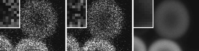
Fig. 2.

Image Quality. Three images of the same specimen (6 μm fluorescent microspheres) are shown. The image on the right has been averaged over 64 scans, while the center and left images were obtained from single scans. Note that although the single scan images appear pixellated, the number of pixels in all the images is the same. The magnified area shown in the top left of each panel demonstrates that there is considerable variability between the images, indicating poor image quality.

Select cells from the specimen by randomly moving the stage and imaging the cell nearest to the center of the field of view if it meets the criteria established in step 1 in Subheading 3.3.

Acquire pairs of images. Replicates of each image are necessary for correlation analysis using RBNCC.

3.4 Display of Colocalization

Overlay the images, using for instance the “Image Color Merge” channels in ImageJ.

Insert one image in the blue layer and display the second image in yellow by inserting it in both the red and green layers, yielding gray or white in areas of similar intensity (see Notes 9 and 10).

A binary display showing colocalized pixels is available in the ImageJ plugin “Colocalization_Finder.”

Scattergrams showing the relationship between the intensities in a pair of images are widely available, including the “Image Correlator” plugin in ImageJ (Fig. 3).

Fig. 3.

Scattergram presenting the overall relationship between the intensities of homologous pixels. For each pixel the intensities in the two channels are used as the coordinates for the scattergram, and the value at that location in the scattergram indicates the incidence of that combination. A perfect correlation would appear as a straight line passing through the origin (if the offset of the detector is accurately set). The slope is not important, since it reflects the gain setting for the two channels, but linearity and the spread are relevant. To select pixels above background, i.e., those with the fluorophore present, a threshold is set for each channel (th1 and th2).

3.5 Measurement of Colocalization

There are a substantial number of similar commercial software packages available for measuring fluorophore colocalization (see Subheading 2.3). User preference and available funds are suggested as issues determining the choice of the appropriate software package.