Comparison of Marginal Space Learning and Full Space Learning in 2D

and Dorin Comaniciu¹

(1)

Imaging and Computer Vision, Siemens Corporate Technology, Princeton, NJ, USA

Abstract

In this chapter, we adapt the Marginal Space Learning to the Left Ventricle (LV) detection in 2D Magnetic Resonance Imaging (MRI) . Furthermore, we compare the performance of the MSL and Full Space Learning. A thorough comparison experiment on the LV detection in MRI images shows that the MSL significantly outperforms the FSL, in both speed and accuracy.

3.1 Introduction

Discriminative learning based approaches have been shown to be efficient and robust for many 2D object detection problems [3, 4, 9, 13, 16]. In these methods, object detection or localization is formulated as a classification problem: whether an image block contains the target object or not. The object is found by scanning the classifier exhaustively over all possible combinations of location, orientation, and scale. As a result, a classifier only needs to tolerate limited variation in object pose, since the pose variability is covered through exhaustive search. Most of the previous methods [3, 9, 13, 16] under this framework only estimate the position and isotropic scaling of a 2D object (three parameters in total). However, in order increase the accuracy of estimation, especially when the object rotates or has anisotropic scale variations, more pose parameters need to be estimated.

In many 2D applications, the task is to estimate an oriented bounding box of the object, which has five degrees of freedom: two for translation, one for orientation, and two for anisotropic scaling. It is a challenge to extend the learning-based approaches to a high dimensional space since the number of hypotheses increases exponentially with respect to the dimensionality of the parameter space. However, a five dimensional pose parameter searching space is still manageable by using a coarse-to-fine strategy . Since the learning and detection are performed in the full parameter space, we call this approach Full Space Learning (FSL) .

The diagram of FSL using the coarse-to-fine strategy is shown in Fig. 3.1. First, a coarse search step is used for each parameter to limit the number of hypotheses to a tractable level. For example, the search step size for position can be set to as large as eight pixels to generate around 1,000 position hypotheses for an image with a size of 300 × 200 pixels. The orientation search step size is set to 20 degrees to generate 18 hypotheses for the whole orientation range. Similarly, the search step size for scales are also set to a large value. Even with such coarse search steps, the total number of hypotheses can easily exceed one million (see Sect. 3.3). Bootstrapping can be exploited to further improve the robustness of coarse detection. In the fine search step, we search around each candidate using a smaller step size, typically, reducing the search step size by half. This refinement procedure can be iterated several times until the search step size is small enough. For example, in the diagram shown in Fig. 3.1, we iterate the fine search step twice.

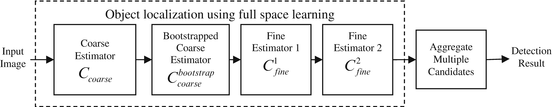
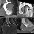
Fig. 3.1

Object localization using full space learning with a coarse-to-fine strategy. ©2009 SPIE. Reprinted, with permission, from Zheng, Y., Lu, X., Georgescu, B., Littmann, A., Mueller, E., Comaniciu, D.: Automatic left ventricle detection in MRI images using marginal space learning and component-based voting. In: Proc. of SPIE Medical Imaging, vol. 7259, pp. 1–12 (2009)

In this chapter, we adapt the MSL to the Left Ventricle (LV) detection in 2D Magnetic Resonance Imaging (MRI) —see Fig. 3.2. Furthermore, we compare the performance of the MSL and FSL. A thorough comparison experiment on the LV detection in MRI images shows that the MSL significantly outperforms FSL, on both the training and test sets.

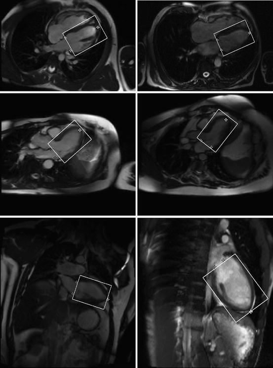
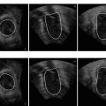
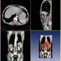
Fig. 3.2

Detection results of the left ventricle (the oriented bounding boxes) and its landmarks (white stars for the left ventricle apex and dark stars for two annulus points on the mitral valve)

The remainder of this chapter is organized as follows. The adaptation of the MSL for LV detection in 2D long axis cardiac MR images is presented in Sect. 3.2. We then present our implementation of the FSL using a coarse-to-fine strategy for LV detection in Sect. 3.3. The quantitative comparison between the MSL and FSL on a large cardiac MR dataset is performed in Sect. 3.4.

3.2 Marginal Space Learning for 2D Object Detection

In this section, we present a 2D object detection scheme using the computational framework of Marginal Space Learning (MSL). The training procedure of 2D MSL is similar to the 3D variant. In the following, we use the LV detection in 2D MRI images as an example to illustrate the whole training workflow. The training parameters (e.g., criteria for positive/negative samples and the number of hypotheses retained after each step in MSL) are given in this section to facilitate the in-depth understanding of the system by the interested reader. For other 2D object detection tasks, the training parameters can be tuned to further improve the detection accuracy. To cope with different scanning resolutions, the input images are first normalized to the 1 mm resolution.

3.2.1 Training of Position Estimator

To localize a 2D object, we need to estimate five parameters: two for position, one for orientation, and two for anisotropic scaling. As shown in Fig. 2.3, we first estimate the position of the object in an image. We treat the orientation and scales as the intra-class variations ; therefore, learning is constrained in a marginal space with two dimensions. Haar wavelet features are very fast to compute and have been shown to be effective for many applications [13]. We also use Haar wavelet features for learning during this step.

Given a set of position hypotheses , we split them into two groups, positive and negative, based on their distances to the ground truth. A positive sample (X, Y ) should satisfy

$\displaystyle{ \max \{\vert X - X_{t}\vert,\vert Y - Y _{t}\vert \}\leq 2\mbox{ mm}, }$

(3.1)

and a negative sample should satisfy

$$$\displaystyle{ \max \{\vert X - X_{t}\vert,\vert Y - Y _{t}\vert \} > 4\mbox{ mm}. }$$ ” src=”/wp-content/uploads/2016/08/A314110_1_En_3_Chapter_Equ2.gif”></DIV></DIV><br /> <DIV class=EquationNumber>(3.2)</DIV></DIV>Here, (<SPAN class=EmphasisTypeItalic>X</SPAN> <SUB><SPAN class=EmphasisTypeItalic>t</SPAN> </SUB>, <SPAN class=EmphasisTypeItalic>Y</SPAN> <SUB><SPAN class=EmphasisTypeItalic>t</SPAN> </SUB>) is the ground truth of the object center. Samples within (2, 4] mm to the ground truth are excluded in training to avoid confusing the learning algorithm. All positive samples satisfying Eq. (<SPAN class=InternalRef><A href=$ 3.1) are collected for training. Generally, the total number of negative samples from the whole training set is quite large. Due to the computer memory constraint, we can only train on a limited number of negatives. For this purpose, we randomly sample about three million negatives from the whole training set, which corresponds to a sampling rate of 17.2 % .

Given a set of positive and negative training samples, we extract 2D Haar wavelet features for each sample and train a classifier using the Probabilistic Boosting-Tree (PBT) [10] . We use the trained classifier to scan a training image, pixel by pixel, and preserve top N ₁ candidates. The number of preserved candidates should be tuned based on the performance of the trained classifier and the target detection speed of the system. Experimentally, we set N ₁ = 1, 000. This number is about 10 times larger than the corresponding parameter for 3D MSL [19, 20] discussed in the previous chapter (3D LV detection application in CT volumes). The reason is perhaps due to more LV shape variability of the slice-based representation and more appearance variability in the case of Cardiac MRI versus Cardiac CT.

3.2.2 Training of Position-Orientation Estimator

For a given image, suppose we have N ₁ preserved candidates, (X _i, Y _i), $i = 1,\ldots,N_{1}$ , of the object position. We then estimate both the position and orientation. The parameter space for this stage is three dimensional (two for position and one for orientation), so we need to augment the dimension of candidates. For each candidate of the position, we sample the orientation space uniformly to generate hypotheses for orientation estimation. The orientation search step is set to be five degrees, corresponding to 72 orientation hypotheses. Among all these hypotheses, some are close to the ground truth (positive) and others are far away (negative). The learning goal is to distinguish the positive and negative samples using image features. A hypothesis (X, Y, θ) is regarded as a positive sample if it satisfies both Eq. (3.1) and

$\displaystyle{ \vert \theta -\theta _{t}\vert \leq 5\mbox{ degrees}, }$

(3.3)

and a negative sample satisfies either Eq. (3.2) or

$$$\displaystyle{ \vert \theta -\theta _{t}\vert > 10\mbox{ degrees}, }$$ ” src=”/wp-content/uploads/2016/08/A314110_1_En_3_Chapter_Equ4.gif”></DIV></DIV><br /> <DIV class=EquationNumber>(3.4)</DIV></DIV>where <SPAN class=EmphasisTypeItalic>θ</SPAN> <SUB><SPAN class=EmphasisTypeItalic>t</SPAN> </SUB>represents the ground truth of the object orientation. Similarly, we random sample three million negatives, corresponding to a sampling rate of 6.6 % on our training set.</DIV><br /> <DIV class=Para>Since the alignment of Haar wavelet features to a specific orientation is not efficient, involving image rotations, we employ the steerable features to avoid such image rotations (see Sect. <SPAN class=ExternalRef><A href=$ 2.3.2 of Chap. 2). A trained PBT classifier is used to prune the hypotheses to preserve only top N ₂ = 100 candidates for object position and orientation.

3.2.3 Training of Position-Orientation-Scale Estimator

The full-parameter estimation step is analogous to position-orientation estimation excepting that learning is performed in the full five dimensional similarity transformation space . The dimension of each candidate is augmented by scanning the scale subspace uniformly and exhaustively. The ranges of S _xand S _yof the LV bounding box are [56.6, 131.3] mm and [37.0, 110.8] mm, respectively, deduced from the training set. The search step for scales is set to 6 mm. To cover the whole range, we generate 14 uniformly distributed samples for S _xand 13 for S _y, corresponding to 182 hypotheses for the scale space.

A hypothesis (X, Y, θ, S _x, S _y) is regarded as a positive sample if it satisfies Eqs. (3.1), (3.3), and

$\displaystyle{ \max \{\vert S_{x} - S_{x}^{t}\vert,\vert S_{ y} - S_{y}^{t}\vert \}\leq 6\mbox{ mm}, }$

(3.5)

and a negative sample satisfies any of Eqs. (3.2), (3.4), or

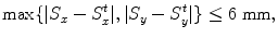
$$$\displaystyle{ \max \{\vert S_{x} - S_{x}^{t}\vert,\vert S_{ y} - S_{y}^{t}\vert \} > 12\mbox{ mm}, }$$ ” src=”/wp-content/uploads/2016/08/A314110_1_En_3_Chapter_Equ6.gif”></DIV></DIV><br /> <DIV class=EquationNumber>(3.6)</DIV></DIV>where <SPAN class=EmphasisTypeItalic>S</SPAN> <SUB><SPAN class=EmphasisTypeItalic>x</SPAN> </SUB><SUP><SPAN class=EmphasisTypeItalic>t</SPAN> </SUP>and <SPAN class=EmphasisTypeItalic>S</SPAN> <SUB><SPAN class=EmphasisTypeItalic>y</SPAN> </SUB><SUP><SPAN class=EmphasisTypeItalic>t</SPAN> </SUP>represent the ground truth of the object scales in <SPAN class=EmphasisTypeItalic>x</SPAN> and <SPAN class=EmphasisTypeItalic>y</SPAN> directions, respectively. Similarly, three million negative samples are randomly selected, corresponding to a sampling rate of 12.0 % on our training set. The steerable features and the PBT are used for training.</DIV></DIV><br /> <DIV id=Sec6 class=$

3.2.4 Object Detection in Unseen Images

This section provides a summary on running the LV detection procedure on an unseen image. The input image is first normalized to the 1 mm resolution. All pixels are tested using the trained position classifier and the top 1,000 candidates, (X _i, Y _i), $i = 1,\ldots,1,000$ , are kept. Next, each candidate is augmented with 72 hypotheses about orientation, (X _i, Y _i, θ _j), $j = 1,\ldots,72$ . The trained position-orientation classifier is used to prune these 1, 000 × 72 = 72, 000 hypotheses and the top 100 candidates are retained, $(\hat{X}_{i},\hat{Y }_{i},\hat{\theta }_{i})$ , $i = 1,\ldots,100$ . Similarly, we augment each candidate with a set of hypotheses about scaling and use the trained position-orientation-scale classifier to rank these hypotheses. For LV bounding box detection, we have 182 scale combinations, resulting in a total of 100 × 182 = 18, 200 hypotheses. For a typical image of 300 × 200 pixels, in total, we test $300 \times 200 + 1,000 \times 72 + 100 \times 182 = 150,200$ hypotheses. The final detection result is obtained using cluster analysis on the top 100 candidates after position-orientation-scale estimation.