COMPUTED TOMOGRAPHY: INTRODUCTION AND GENERAL PRINCIPLES

ANTHONY A. MANCUSO, MANUEL ARREOLA, AND SURESH K. MUKHERJI

KEY POINTS

Basis of computed tomography spatial resolution
Basis of computed tomography contrast resolution
Computed tomographic angiography techniques and uses
Intravenous iodinated contrast use
Factors affecting protocol development and imaging strategy choices in clinical practice
Speculative value of computed tomography perfusion techniques outside of the brain

Systems capable of routinely producing excellent images of the entire head and neck region have been generally available since 1985. In the early to mid 1990s, there was a revolution in computed tomography (CT) technology. This started in the early 1990s with slip-ring technology that permitted continuous motion of the x-ray tube and detector array, which led to multislice acquisition capabilities in the late 1990s. That began the volume acquisition era circa 2001 to 2006. These capabilities continue to grow and with the dynamic volume acquisition capability of the 320 multidetector computed tomography (MDCT) that arrived in the spring of 2008 now provide physiologic motion, blood flow, and perfusion data.

The continuous-motion CT scanner was a major advance in technology that profoundly affects the efficiency of the modality and expands the amount of diagnostic information produced. The related slip-ring gantry allowed the tube to rotate continuously while the patient table moved, whether the unit was either of third- or fourth-generation configurations. This capability allowed CT to produce a volumetric projection acquisition. In addition, multislice dynamic CT, the forerunner of computed tomographic angiography (CTA) and perfusion studies, became a viable approach for routine rudimentary CT acquisition of such data.

True volumetric CT required hardware in addition to that of the slip-ring (continuous-motion) gantry. This hardware included the following:

(1) An x-ray tube with increased heat storage and dissipating capacity since the continuous rotation of the tube demands that the tube be operating at high currents while it is on continuously

(2) Improved detection systems, the most recent being the 320 MDCT detector that essentially acts as a rotating flat panel albeit with the resolution of a CT detector rather than that of a flat panel

(3) A patient table capable of high-precision stepping (i.e., submillimeter tolerance) reliably synchronized with tube rotation

(4) Computer hardware that allows for extensive multitasking (parallel and/or distributive processing)

Extensive new software has been developed to take advantage of all data available in a volumetric acquisition. This software is now routinely available on workstations built by either the scanner manufacturers or by others.

There are several potential advantages to the rapid acquisition of volumetric CT data. These include the following:

(1) Increased throughput: A basic set of 100 to 2,500 images through the head and neck can be acquired, processed and reviewed, and stored in 4 to 5 minutes. Assuming 5 to 10 minutes of positioning and preparation time on the table, a routine head and neck total examination time should not exceed 15 minutes. Faster studies are especially helpful in pediatric and trauma patients and are indispensable for CTA and perfusion studies.

(2) Since the area of interest is studied so rapidly, the volume of contrast needed for extracranial CT studies has been marginally reduced by about 25%, which permits a modest cost savings.

(3) Effects of both voluntary and involuntary patient motion can be minimized; this has a greater impact in body rather than on head and neck studies.

(4) Some basic functional analysis, such as vocal cord motion or dynamic changes in the airway that might be present in tracheomalacia or sleep apnea, may be done; this usage will increase with the new 320 MDCT units and future iterations of the advancing detector development cycle.

(5) z-axis resolution improves dramatically since the volumetric data can be fully exploited multidirectionally in the reconstruction algorithm. This makes very high-quality multiplanar reformation possible. The improved raw data in the volume set also improves the quality of three-dimensional (3D) images.

Basic requirements for good head and neck CT imaging are as follows:

(1) Slice thickness (SLT): 0.5 to 1.0 mm for high-detail work; 2.0 to 3.0 mm for routine studies not requiring reformations

(2) Field of view (FOV): 7 to 18 cm

(3) Matrix: 512 × 512.

(4) CT angiographic capabilities (≥16-slice MDCT, although rudimentary CTA can be done on a 4-slice MDCT); true 256 to 320 MDCT to allow study of flow dynamics and angioarchitecture with an adequate z-axis area of coverage

The limitations of spatial and contrast resolution in any CT system are fundamentally influenced by original projection data measurements. Primary factors inherent to the particular CT system utilized are related to hardware geometry and characteristics influencing projection data measurement. These are dependent on the geometry of the unit and the related hardware. These factors include focal spot size, aperture width, detector element size, geometry, and detective quantum efficiency. Proper specification of these parameters through a request for proposal at the time of purchase of the CT equipment can ensure that these parameters are appropriately chosen. Other factors affecting spatial and contrast resolution relate to the choice of imaging parameters generically referred to as the “technique” and are commonly under operator control. Many of these factors should be determined in preprogrammed imaging protocols. These factors greatly influence the information content of the image if one pays attention to a few simple details during the planning stages of each examination (Appendix A). These include beam energy (peak kilovoltage [kVp]) and intensity or fluence (milliamperes [mA]), SLT (as a function of collimation and speed of table motion), matrix size, reconstruction FOV, and choice of reconstruction algorithm as well as the strategic use of intravenous (IV) contrast enhancement.

SPATIAL RESOLUTION

In CT, changes in imaging parameters that decrease voxel size result in reduced photon fluences per voxel and decreased signal-to-noise ratio (SNR). This in turn decreases image contrast while improving spatial resolution, as smaller pixels are utilized. In a given situation, one must consider whether to increase the number of photons per voxel (milliamperes per second) to compensate for this loss in SNR. This decision will largely depend on the inherent subject contrast and size of the region or pathology under study. The main cost of increased milliamperes per second is the increased patient exposure. For instance, an adult study of the temporal bone at higher milliamperes per second may look better than one done at lower milliamperes, but the lower milliamperes per second examination may be as highly spatially resolved, contain the same diagnostic information, and be more appropriate in a pediatric patient. Increased milliamperes per second actually have relatively little effect on improving resolving power for high-contrast structures such as the temporal bone once a certain threshold is reached. Increasing the milliamperes per second beyond a certain point may improve the appearance of an image, but it probably will not alter diagnostic capabilities. However, if that same pediatric temporal bone study is utilized for brain purposes as well as bone detail, an increase in either the milliamperes per second or the section thickness will improve the low-level contrast detectability.

Trade-offs between patient exposure and spatial and contrast resolution, in a particular region under study, should be determined in advance. Then, study protocols or guidelines should be established based on the individual equipment available and the perceived requirements for the degree of image clarity required for diagnosis. With the currently available tube-detector systems, high-quality, fast images are virtually routine at reasonable dose levels. All CT manufacturers now offer various types of tube current modulation in their scanners to help find the right balance between dose and optimal image quality. In the following sections, it should be apparent that the factors affecting spatial resolution are largely under operator control and may be manipulated to optimize the clarity and information content of the image.

Slice Thickness

Neuroradiologic and head and neck imaging was the driving force behind the move to thinner CT sections in the late 1970s. This move was based upon the need to visualize increasingly small structures, some on the order of a millimeter in size, and a desire for highly resolved reformatted images.

It is known that use of a thinner section results in higher contrast and better spatial resolution for objects not occupying the full thickness of the section because of diminished volume averaging. Reduced section thickness also reduces photon fluence per voxel, and the decreased SNR aggravates the tendency for the system to produce artifacts, such as the aliasing artifacts most commonly visually expressed as bright and dark streaks in the image. The disadvantages of thinner sections are, therefore, potentially noisier images and more artifacts. In areas of high inherent or subject contrast, the increased noise is less problematic because contrast in voxels at the edges of neighboring structures of interest is likely to be far above background noise. The air-bone-soft tissue interfaces of the temporal bone are an ideal situation for the use of thin sections. These interfaces are at the border of small structures that need to be resolved and that have very high inherent contrast. This means that high-contrast images can be obtained using thin sections without dramatically increasing radiation exposure to the patient, assuming that sampling frequency (detector density, time) is adequate to limit artifacts. If thin sections (0.5 to 1.0 mm) are used to study tissues of less inherent contrast such as the brain, then more photon fluence (milliamperes per second) may be required to provide the necessary SNR (Fig. 2.1). If streak artifacts are the problem, an increase in scanning time or sampling frequency by slowing table movement may be more appropriate. A trade-off of increasing the scan time will increase the risk of motion artifacts in uncooperative patients. CT and magnetic resonance images are similar to all other imaging modalities in that optimal spatial and contrast resolution most often require compromises between multiple factors that may tend to work against each other.

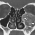
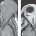
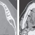
FIGURE 2.1. Images showing the effects of reduction in slice thickness on tissue contrast. A, B: Contrast-enhanced computed tomography images of a mass in the retrostyloid parapharyngeal space (arrow) that shows little if any enhancement. In (A), the section thickness is 3 mm; in (B), the section thickness is 1 mm. There is an obvious reduction in the low-contrast resolution, probably best appreciated by comparing the spinal cord within the subarachnoid space on the two images (arrowheads). However, the decrement in tissue contrast resolution has no significant effect on the evaluation of the mass or its relationship to surrounding structures. In looking at the skeletal musculature, it is obvious that the image in (B) is significantly noisier than that in (A) due to the reduction in voxel size. C, D: The effects of reduction in slice thickness on a contrast-enhancing abnormality of the pharyngeal walls. In (C), the section thickness is 3 mm; in (D), the section thickness is 1 mm. Part (D) is obviously noisier, but there is no significant decrement in the diagnostic information available in these areas of relatively high inherent contrast.

Another equally important factor is the relationship between the overall cephalocaudal extent of the area under study and the SLT. For instance, it is optimum to have a maximum of 1- to 2-mm sections through the entire larynx and neck. Such routine 100- to 200-slice studies had been considered impractical even in the recent past. As data acquisition and display capabilities have improved, this issue has become trivial. In the upper aerodigestive tract and neck, contiguous 2.5- to 3.0-mm sections are currently adequate for survey at sites of high risk for pathologic involvement. Specific protocols in Appendix A suggest particular adjustments used for particular diagnostic problems in each head and neck anatomic area of interest.

One- or 2-mm contiguous sections are now frequently reconstructed over the portion of the anatomy likely to most critically affect diagnosis and management and/or whenever multiplanar reconstructions or reformations are necessary. These sections may be reconstructed from an acquisition volume data set made with a nominal section thickness of 0.50 to 0.75 mm. The 0.5- to 1.0-mm raw data files must be used if reformation or 3D images are critically important in clinical decision making, such as in studies done for CTA or temporal bone and when looking for areas of dehiscence of bone along the cribriform plate as a cause of cerebrospinal fluid leakage or subtle bone destruction by a cancer. One- to 3-mm sections are important in large as well as small lesions, since it is often the anatomic distortions at the margin of the lesion that will critically alter staging and planning of therapy. On MDCT equipment, extracranial tissue contrast remains good with 0.5- to 1.0-mm sections, with acceptable radiation exposure levels (Fig. 2.1). The temporal bone is always studied with 0.40- to 0.75-mm contiguous sections. The 0.5- to 1.0-mm sections are also appropriate for indications such as detailed evaluation of the facial bones, including the mandible and teeth and skull base as well as orbital (optic nerves) and laryngeal lesions. There is no longer a reasonable deterrent to reconstructing the thinnest possible sections if they are necessary for optimal patient care. Otherwise, 1- to 3-mm sections are appropriate in most other protocols, assuming CTA is not necessary.

Pixel Size: Field of View and Matrix

Reconstruction matrix size is a prime determinant of pixel size. The standard matrix has been 512 × 512 since the mid 1980s. Larger matrices would add burden to digital storage systems without additional diagnostic benefit.

The selection of the FOV is the second major factor affecting pixel size and therefore spatial resolution. The x, y dimensions of a pixel can be derived by dividing the FOV by the matrix size. If a 512 × by 512 matrix and a 12- to 18-cm FOV are used routinely, pixel size should only occasionally exceed 0.25 to 0.35 mm in head and neck studies.

CT voxels are always anisotropic due to z-axis (slice thickness) issues. Some manufacturers like to represent that CT voxels can be made isotropic. Simple arithmetic shows this not to be true, even theoretically or virtually as they would like you to believe, in head and neck work. The 512 × 512 matrix divided by the typical FOV range of CT reconstructions of 9 (for temporal bone) to 16 cm (facial and general neck work) gives a range of about 0.18 to 0.30 mm for the x and y dimensions of the pixel. The nominal 0.400- to 0.625-mm segmentation of current MDCT detectors obviously exceeds those dimensions. Sections can be reconstructed at half the detector segmentation distance, but that still exceeds the usual pixel dimension with a 16-cm FOV, which is about the largest used in high-quality head and neck imaging outside of the FOV of 20 cm typically used to study the brain. Data from volume acquisition can approach the isotropic goal, but it does not meet such a specification (Fig. 2.2). Practically speaking, this may make no difference in diagnostic capability.

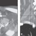
FIGURE 2.2. Temporal bone computed tomography demonstrating the importance of selecting the appropriate field of view for an imaging study depending on the degree of spatial resolution combined with the area of coverage necessary. Also, this study demonstrates the importance of choosing the proper reconstruction algorithm for the job. The field of view chosen was 9.0 cm to optimize spatial resolution; the slice thickness was 0.5 mm. In this area of high inherent contrast, the relatively small voxel size produces an optimal data set for multiplanar anatomic evaluation. A: This patient clinically had a blue mass (arrow) seen through the tympanic membrane. The mass on axial sections is likely contiguous with the jugular fossa. As can be seen from the orthogonal coronal reformation in (B) and the off-axis reformation in (C), the mass is clearly shown as a small jugular diverticulum (arrowhead) projecting into the middle ear from the jugular bulb (arrows). (NOTE: This voxel size is not anywhere near isotropic, but the resolution is certainly adequate in the z-axis to provide a definitive data set for the multiplanar evaluation of the temporal bone.)

Only gold members can continue reading. Log In or Register to continue