Fig. 1
A typical short axis cardiac MR image containing LV, RV and papillary muscles
There have been extensive researches such as graph cuts [4, 5], morphological operations [6, 7], dynamic weights fuzzy connectedness framework [8, 9], active contours or snake model [3, 10–14] and supervised learning methods [15–18], to overcome challenges of the LV segmentation. Petitjean and Dacher [19] presented a comprehensive review of LV segmentation algorithms. Among approaches mentioned above, the snake model is one of the most successful methods, which deforms a closed curve using both the intrinsic properties of the curve and the image information to capture the boundaries of the region of interest (ROI). However, the information (e.g. intensity, texture) only deriving from the image itself is not sufficient to get satisfactory segmentation results. The prior knowledge concerning the LV, therefore, is necessary to be incorporated into the snake model.
In this work, we address the segmentation of the LV focusing on the following challenges: (1) image inhomogeneity; (2) effect of papillary muscle; and (3) weak edges. Our strategy is the employment of the anatomical shape of the LV, rather than the constraints derived from a finite training set. The proposed method is based on the parametric snake model, in which the external forces include the gradient vector flow (GVF) and the proposed gradient vector convolution (GVC). The GVC model can be implemented in real time due to its convolutional nature and possesses similar properties of the GVF model. Considering the LV is roughly a circle, a circle-shape based energy is introduced into the snake model to extract the endocardium of the LV. The circle shape energy is also employed for epicardium segmentation. The ellipse constraint is employed for segmenting the LV as well. The drawback of the ellipse constraint is that one has to estimate the orientation of the ellipse during snake evolution. Assuming the epicardium resembles the endocardium in shape, we further develop a shape-similarity energy functional to prevent the snake contour from leaking out from weak boundaries. With the circle constraint and shape similarity energy, we can extract the endocardium and epicardium of the LV robustly and accurately. This work is based on our approaches presented in [13, 20–23].
2 Related Work
In this study, we address the shape constraints for segmentation of the LV from cine MRI based on snake models. We define intensity, texture or color statistics as weak prior. The prior shape obtained from a training set or from anatomical information (e.g., circle, ellipse) is regarded as strong prior. Based on these principles, in this section, we classify the relevant literature as no prior, weak prior and strong prior to review.
2.1 LV Segmentation Without Prior
The studies falling into this category have mainly concentrated on the design of the external energy. Ranganath [24] tracked the LV endocardium in cardiac MRI sequences by propagating the conventional snake from one frame to another. Makowski et al. [25] employed the balloon snake [26] to extract the LV endocardium and introduced an antitangling strategy to exclude the papillary muscles. The balloon force is defined as
where  is the normal unit vector to the curve at point
  and
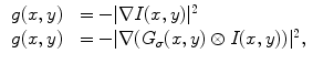
and  is the amplitude of the force. If we change the sign of
  or the orientation of the curve, it will have an effect of deflation instead of inflation. The curve expands and it is attracted and stopped by edges as before, but since there is a pressure force, if the edge is too weak the curve can pass through this edge. Therefore, it is prone to lead to weak edge leakage during LV segmentation. Based on the discrete contour model, Hautvast et al. [27] developed a method that attempts to maintain a constant contour environment in the vicinity of the cavity boundary. Due to the high performance at capture range enlarging, the gradient vector flow (GVF) snake [28] has been employed for the LV segmentation [29], but Santarelli et al. [29] did not consider the effect of weak boundaries, papillary muscle and artifacts stemming from swirling blood. It is also not clear how the GVF snake model captured the epicardium soon after the endocardium was extracted. The GVF field
 ![$$\varvec{V}(x,y)=\left[ u(x,y),v(x,y)\right] $$](/wp-content/uploads/2016/10/A312883_1_En_12_Chapter_IEq5.gif) is defined as
is defined as
![$$\begin{aligned} E(u,v) = \int \!\!\!\!\int \ \Big [\mu \left( u_{x}^{2}+u_{y}^{2}+v_{x}^{2}+v_{y}^{2}\right) + |\nabla {f}|^{2} |\varvec{ V}-\nabla {f}|^{2}\Big ] d x d y . \end{aligned}$$](/wp-content/uploads/2016/10/A312883_1_En_12_Chapter_Equ2.gif)
The behavior of the GVF will be discussed in Sect. 3.2. Lee et al. [30] presented the iterative thresholding method to extract the endocardium, which effectively alleviates the interference of papillary muscle. However, the endocardial contour is not smooth enough and the movement constraint based on image intensity for the snake is too empirical. Nguyen et al. [31] compared the conventional snake, balloon snake and GVF snake on extracting the LV endocardium and concluded that the GVF snake has the best performance.
(1)
is the normal unit vector to the curve at point and is the amplitude of the force. If we change the sign of or the orientation of the curve, it will have an effect of deflation instead of inflation. The curve expands and it is attracted and stopped by edges as before, but since there is a pressure force, if the edge is too weak the curve can pass through this edge. Therefore, it is prone to lead to weak edge leakage during LV segmentation. Based on the discrete contour model, Hautvast et al. [27] developed a method that attempts to maintain a constant contour environment in the vicinity of the cavity boundary. Due to the high performance at capture range enlarging, the gradient vector flow (GVF) snake [28] has been employed for the LV segmentation [29], but Santarelli et al. [29] did not consider the effect of weak boundaries, papillary muscle and artifacts stemming from swirling blood. It is also not clear how the GVF snake model captured the epicardium soon after the endocardium was extracted. The GVF field is defined as(2)
However, the information (e.g. intensity, texture) only derived from the image itself is not sufficient to get satisfactory segmentation results. It is difficult to deal with the noisy and incomplete data. The prior knowledge concerning the anatomy, appearance and motion of the LV, therefore, is necessary to be incorporated into the snake model. The prior information may be the statistical shape from a training set [11, 32, 33], be anatomical information such as ellipse in [34–36], or be intensity, texture or color statistics [37, 38].
2.2 LV Segmentation with Weak Priors
Lynch et al. [39] presented a novel and intuitive approach to combine 3-D spatial and temporal MRI data in an integrated segmentation algorithm to extract the myocardium of the left ventricle. By encoding prior knowledge about cardiac temporal evolution, an EM algorithm optimally tracks the myocardial deformation over the cardiac cycle. Punithakumar et al. [38] presented an original information theoretic measure of heart motion based on the Shannon’s differential entropy (SDE), which allows heart wall motion abnormality detection. Folkesson et al. [33] extended the geodesic active region method by incorporating the statistical classifier for segmentation of cardiac MRI. Paragios [32] integrated visual information with anatomical constraint into the variational level set approach [40].
Ayed et al. [12] proposed to derive the curve evolution equations by minimizing two functionals each containing an original overlap prior constraint between the intensity distributions of the cavity and myocardium. This overlap prior constraint largely improves the segmentation accuracy and enhances the robustness of the algorithm. For each region  , define
  as the nonparametric (kernel-based) estimate of intensity distribution within region
  in frame
where  is the area of region
Ayed et al. [12] assume that a segmentation of the first frame  , i.e., a partition
  is given. The amount of overlap between the intensity distribution within the heart cavity region in
  and the myocardium model learned from the first frame, is formulated as
Similarly, the background model learned from the first frame is given by
Mean-matching terms measures the conformity of intensity means within the cavity and the myocardium in the current frame to mean priors learned form the first frame
where
The gradient terms is defined as
where  is a positive constant and
  is an edge indicator. The functionals to minimize are a weighted sum of the three characteristic terms (i.e., overlap prior terms, mean-matching terms and gradient terms) given by
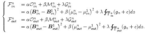
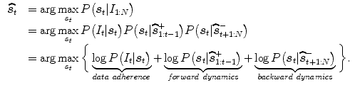
To relax the dependence on the choice of a training set, Zhu et al. [41] build subject-specific dynamic model from a user-provided segmentation of one frame in the current cardiac sequence, which is able to simultaneously handle temporal dynamics (intrasubject variability) and intersubject variability. The Bayesian framework combining the forward and backward segmentation is expressed as
Ayed et al. [3] introduced a novel max-flow segmentation of the LV by recovering subject-specific distributions learned from the first frame via a bound of the Bhattacharyya measure. The total cost function is given by
![$$\begin{aligned} \begin{array}{ll} \arg \min \limits _{L:P\rightarrow 0,1} \Bigg [ &{}-\sum \limits _{i \in I}\sqrt{\varvec{P}_{L,I^{n}}(i) {\mathcal {M}}_{\varvec{c},I}(i)} - \sum \limits _{d \in D}\sqrt{\varvec{P}_{L,D^{c}}(d) {\mathcal {M}}_{\varvec{c},D}(d)} \\ &{}+\sum \limits _{\{ p,q \} \in {\mathcal {N}}} \frac{1}{||p-q||} \delta _{L(p)\ne L(q)} \Bigg ], \end{array} \end{aligned}$$](/wp-content/uploads/2016/10/A312883_1_En_12_Chapter_Equ12.gif)
where  is the learned model distribution of intensity and
  is the model distribution of distances within the cavity in the first frame. Jolly et al. [42] combined the edge, region and shape information to extract the LV endocardium, the approximate shape of the LV is obtained based on the maximum discrimination method. They used the shape alignment method proposed by Duta et al. [43] to establish the correspondence between a subset
  of the template points and a subset
  of the candidate points. The goal of shape constraint in [42] is to find the coefficients
  of the similarity transform which minimize the distance
  .
.
![$$\begin{aligned} \begin{array}{ll} f(N_{c}) =&{} \frac{1}{N_{c}^{2}} \sum \limits _{j=1}^{N_{c}} w(B_{j}) \bigg [ \big ( x_{A_{j}}- a x_{B_{j}} -c y_{B_{j}} -b \big )^{2} \\ &{}+ \big ( y_{A_{j}}- a y_{B_{j}} -c x_{B_{j}} - d \big )^{2}\bigg ] + \frac{2}{N_{c}}, \end{array} \end{aligned}$$](/wp-content/uploads/2016/10/A312883_1_En_12_Chapter_Equ13.gif)
where  is the number of established correspondence.
, define as the nonparametric (kernel-based) estimate of intensity distribution within region in frame (3)
is the area of region (4)
, i.e., a partition is given. The amount of overlap between the intensity distribution within the heart cavity region in and the myocardium model learned from the first frame, is formulated as(5)
(6)
(7)
(8)
(9)
is a positive constant and is an edge indicator. The functionals to minimize are a weighted sum of the three characteristic terms (i.e., overlap prior terms, mean-matching terms and gradient terms) given by(10)
(11)
(12)
is the learned model distribution of intensity and is the model distribution of distances within the cavity in the first frame. Jolly et al. [42] combined the edge, region and shape information to extract the LV endocardium, the approximate shape of the LV is obtained based on the maximum discrimination method. They used the shape alignment method proposed by Duta et al. [43] to establish the correspondence between a subset of the template points and a subset of the candidate points. The goal of shape constraint in [42] is to find the coefficients of the similarity transform which minimize the distance .(13)
is the number of established correspondence.2.3 LV Segmentation with Strong Priors
As shown by the growing literature on the LV segmentation, it benefit from the use of an anatomical constraint (e.g., shape model) on active contour model to enhance the robustness and accuracy of the segmentation. Pluempitiwiriyawej et al. [35] incorporated the ellipse constraint into the segmentation scheme. However, there should be an isolated step to estimate the five parameters of the ellipse, which does not comply with the evolution of the snake contour.
The atlas warping technique introduced by Lorenzo-Valdes et al. [44] is a typical training-based method, the atlas is constructed from manually segmented and temporally aligned data and is registered on the data for automatic segmentation. This algorithm is based on the 4D extension of expectation maximization (EM) algorithm. The active shape model (ASM) first proposed by Cootes et al. [15] is constructed from a training set of segmented objects using the principal component analysis (PCA) algorithm. The ASM minimizes the difference between the synthesized image from the model and an unseen image by tuning the model parameters, when it is applied to image interpretation or segmentation. Assen et al. [45] applied 3D-ASM to image data sets with an increasing sparsity comprising images with different orientations and stemming from different MRI acquisition protocols. Later, Assen et al. [46] investigated the effect of initialization on segmentation results in [45] and proposed a semiautomatic segmentation method of cardiac CT and MR volumes, without the requirement of retraining the underlying statistical shape model.
The active appearance model (AAM) is extended from the ASM by taking into account the intensity distribution in the training set [16, 47]. AAM is able to simultaneously describe the shape and texture variation of objects. The AAM is more robust than the ASM when the intensity contrast is low and the object boundary is weak. There has been a great diversity of works devoted to the construction and application of the ASM/AAM models, particularly for the extraction of the LV from cardiac MRI. Gopal et al. [48] applied AAM and deformable superquadric models to automate the segmentation of the LV in cardiac MR cine images for the end-diastole and end-systole phases, in which the texture model in the AAM is modified by radially sampling gradient magnitude values. Ghose et al. [49] applied 2D AAM with a 3D shape restriction imposed by rigidly registering the obtained volume to a 3D average model of the prostate. Mitchell et al. [50] devised a multistage hybrid active appearance model (AAM) by combining ASM and AAM. Pfeifer et al. [51] used a 2D AAM for the blood mass of left and right ventricle and an additional three division 2D AAM to cope with the shape variation of the blood mass of the left and right ventricle. Zambal et al. [52] combined AAM and ASM for the LV segmentation, in which the global model construction interconnects a set of 2D AAM by a 3D shape model. Recently, Zhang et al. [17] also combined the ASM and AAM but to construct a biventricular model to segment the left and right ventricles simultaneously. Although excellent results have been achieved in [45, 48, 51, 52] where the LV shape is learned from an annotated training data set, the segmentation performance depends heavily on the size and richness of images in the training set.
3 Background: Active Contours
3.1 Tranditional Active Contours
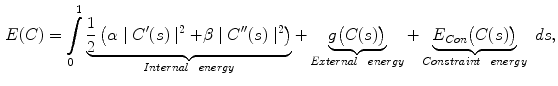
Active contour models, or snakes [10], have been proven to be very effective tools for image segmentation. It integrates an initial estimate, geometrical properties of the contour, image data and knowledge-based constraints into a single process, and provides a good solution to shape recovery of objects of interest in visual data. A traditional active contour model is represented by a curve 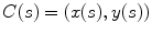 ,
, ![$$s\in [0,1]$$](/wp-content/uploads/2016/10/A312883_1_En_12_Chapter_IEq25.gif) . It moves through the spatial domain of an image to minimize the energy functional
. It moves through the spatial domain of an image to minimize the energy functional
where  and
and  denote the first and second derivatives of
  with respect to
  , respectively. The first term of the integral stands for the internal force that keeps the contour continuous and smooth during deformation, the second term is the external force that drives the contour toward an object boundary or the other desired features within an image. The constraint energy term
  is derived from the prior information (e.g., in this chapter, we concentrate on designing a novel constraint energy by considering the anatomical information of the LV to enhance the robustness and accuracy of the LV segmentation). The external energy function
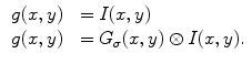
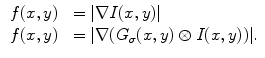
  is derived from the image so that it takes on its smaller values at the features of interest, such as boundaries. Given a gray-level image
  , typical external energies are defined as follows,
where  is a two-dimensional Gaussian function with standard deviation
  ,
,  is the gradient operator, and
  is convolution operation. If the image is a line drawing (black and white), then appropriate external energies include
By using the calculus of variation, the Euler equation to minimize  is
is

According to the representation and implementation, active contour models are classified into two categories: the parametric active contour models [26, 28, 53] and the geometric active contour models [54–57]. In this paper, we focus on the parametric active contour models, and our approach can be also integrated into geometric active contour models. Since the external force plays a leading role in driving the active contours to approach objects boundaries in the parametric active contour models, designing a novel external force field has been extensively studied [26, 28, 58–61]. Among all these external forces, gradient vector flow (GVF) proposed by Xu and Prince [28], has been one of the most successful external forces, which is computed as a diffusion of the gradient vectors of a gray-level or binary edge map derived from a given image to increase the capture range. Due to the outstanding properties of GVF, a large number of modified versions have been presented [58, 60, 62, 63] to improve the performance of active contour models. However, researchers found that the GVF suffers from several challenges including narrow and deep concavity convergence as well as weak edge leakage. In the next section, we elaborate the behavior of the GVF snake model.
, . It moves through the spatial domain of an image to minimize the energy functional(14)
and denote the first and second derivatives of with respect to , respectively. The first term of the integral stands for the internal force that keeps the contour continuous and smooth during deformation, the second term is the external force that drives the contour toward an object boundary or the other desired features within an image. The constraint energy term is derived from the prior information (e.g., in this chapter, we concentrate on designing a novel constraint energy by considering the anatomical information of the LV to enhance the robustness and accuracy of the LV segmentation). The external energy function is derived from the image so that it takes on its smaller values at the features of interest, such as boundaries. Given a gray-level image , typical external energies are defined as follows,(15)
is a two-dimensional Gaussian function with standard deviation , is the gradient operator, and is convolution operation. If the image is a line drawing (black and white), then appropriate external energies include(16)
is(17)
3.2 GVF Snake Model
Notwithstanding the marvelous ability in representing object shapes, the traditional active contour model is limited to capture range and poor convergence to boundary concavities. Gradient vector flow (GVF) was proposed by Xu and Prince [28] as a new external force for active contour model to overcome these issues. It is a dense vector field, generated by diffusing the gradient vectors of a gray-level or binary edge map derived from an image. The GVF field is defined as a vector field ![$$\varvec{V}(x,y)=\left[ u(x,y),v(x,y)\right] $$](/wp-content/uploads/2016/10/A312883_1_En_12_Chapter_IEq38.gif) that minimizes the following energy functional:
that minimizes the following energy functional:
![$$\begin{aligned} E(u,v) = \int \!\!\!\!\int \ \Big [\mu \left( u_{x}^{2}+u_{y}^{2}+v_{x}^{2}+v_{y}^{2}\right) + |\nabla {f}|^{2} |\varvec{ V}-\nabla {f}|^{2}\Big ] d x d y , \end{aligned}$$](/wp-content/uploads/2016/10/A312883_1_En_12_Chapter_Equ18.gif)
where  is the edge map defined as
 is high near the edges and nearly zero in homogeneous regions and
  is a positive weight to control the balance between smoothness energy and edge energy. We see that when
  is small, the energy is dominated by sum of the squares of the partial derivatives of the vector field, yielding a slowly-varying field. On the other hand, when
  is large, the second term dominates the integrand and minimized by setting
  . This produces the desired effect of keeping
  nearly equal to the gradient of the edge map when it is large, but forcing the field to be slow-varying when in homogeneous regions.
that minimizes the following energy functional:(18)
is the edge map defined as(19)
is high near the edges and nearly zero in homogeneous regions and is a positive weight to control the balance between smoothness energy and edge energy. We see that when is small, the energy is dominated by sum of the squares of the partial derivatives of the vector field, yielding a slowly-varying field. On the other hand, when is large, the second term dominates the integrand and minimized by setting . This produces the desired effect of keeping nearly equal to the gradient of the edge map when it is large, but forcing the field to be slow-varying when in homogeneous regions.By the calculus of variation, the minimization of Eq. (18) reduces to solving the following Euler-Lagrange equation:
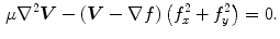
The Euler-Lagrange equations evolving Eq. (20), embedded into a dynamic scheme by treating  as the function of
  ,
,  and
and  , formally are
where  is the Laplacian operator. The active contour model with
  as external force is called GVF active contour model.
(20)
as the function of , and , formally are(21)
is the Laplacian operator. The active contour model with as external force is called GVF active contour model.GVF has successfully addressed the issues of building a satisfactory capture range and approaching boundary concavities, e.g., U-shape concavity convergence. However the GVF active contour model still fails to converge to narrow and deep concavity and would leak out around weak edges, especially neighbored by strong ones. More importantly, the computational cost of the GVF model is very high. In the next Section, we will elaborate the calculation of the GVF.
4 A New External Force: Gradient Vector Convolution
4.1 Computational Analysis of the GVF
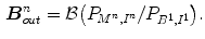
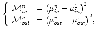
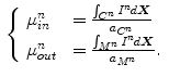
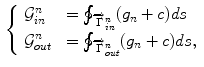
The computation of a GVF field consists mainly of solving a huge discretized system of partial differential equations, which has restricted its potential applications to images with large sizes. Among the general numerical implementation of the GVF filed, diffusion is an iterative technique that depends upon a termination time. This involves how to choose an optimal iteration number in diffusion process. As discussed in [28] ,“the steady-state solution of these linear parabolic equations is the desired solution of the Euler equations … ,” this statement gives rise to the following question: dose “the desired solution of the Euler equations” be the desired external force for Snake model, i.e., the desired GVF? We answer this question and demonstrate the influence of iteration number in Fig. 2. GVF fields at 100, 200 and 2000 iterations of diffusion are given in Fig. 2a–c respectively. Visibly, the result in Fig. 2c is far from available in that the GVF flows into the ventricle from right and out from left-bottom depicted in the white rectangle. Surely, the result in Fig. 2c approximates the steady state solution, but it cannot serve as the external force for snake model. The reason behind this situation is that Eq. (21) is a biased version of  by
by  , where
  is an isotropic diffusion. As
  increases, the isotropic smoothing effect will dominate the diffusion of Eq. (21) and converge to the average of the initial value. Small enough
  could depress this oversmoothing efficacy, but, at the same time, preserves excessive noise. Alternatively, an optimal iteration number, say,
  for this example, would be an effective solution for this issue, however, it is still computationally expensive.
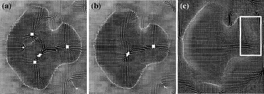
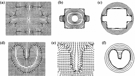
by , where is an isotropic diffusion. As increases, the isotropic smoothing effect will dominate the diffusion of Eq. (21) and converge to the average of the initial value. Small enough could depress this oversmoothing efficacy, but, at the same time, preserves excessive noise. Alternatively, an optimal iteration number, say, for this example, would be an effective solution for this issue, however, it is still computationally expensive.Fig. 2
Gradient vector flow fields at different iteration: a GVF at  iteration; b GVF at
  iteration; c GVF at
  iteration. The white dots represent critical points of the flow field [22]. The parameters of GVF are
  , time step
iteration; b GVF at iteration; c GVF at iteration. The white dots represent critical points of the flow field [22]. The parameters of GVF are , time step One possible solution is to develop alternative external forces which can be efficiently computed. For example, Park and Chung [64] and Yuan and Lu [65] simultaneously proposed the virtual electric field (VEF) based external force, in which each pixel is considered as a static charge. The VEF possesses the advantage of being implemented in real time over the GVF while maintaining other desirable properties such as large capture range and concavity convergence. Jalba et al. [66] recently proposed the charged particle model, where each pixel is also considered as static charge. The authors demonstrated that the particles could be initialized randomly across the image and did not suffer from convergence issues related to GVF/GGVF. Li and Acton et al. [67] proposed convolving the image edge map with a vector field kernel, which comprises radial symmetric vectors pointing towards the center of the kernel.
Another solution is to design efficient numerical schemes for fast GVF computation. Vidholm et al. [68] employed the preconditioned conjugate gradient methods and multigrid methods to accelerate the computation of 3D GVF fields. Han et al. [69] proposed a multigrid GVF/GGVF algorithm, which can significantly improve the computational efficiency. Boukerroui [70] compared several efficient numerical schemes for GVF computation, and showed that the alternating direction explicit scheme (ADES) may be a suitable alternative to the multigrid method. Ren et al. [71] presented methods for fast GVF and GGVF computation by combining the augmented Lagrangian method and multiresolution scheme.
To overcome issues mentioned above, we argue that one can extend the gradient vector and suppress noise by convolving the gradient vector with a certain kernel. To this end, a convolution-based external force called gradient vector convolution (GVC) will be introduced in Sect. 4.2. Due to the fast fourier transform, the convolution operation would be implemented in real time and the snake model would benefit much from this convolution operation in computation time. The GVC method possesses some advantages of the GVF such as enlarged capture range, initialization insensitivity, concavity convergence, but its computational cost is low owing to its convolution mechanism. Some experiments are presented to demonstrate these advantages in Sect. 4.2.
4.2 Gradient Vector Convolution External Force
For any bounded  , the linear diffusion process
  ,
,  possesses the unique solution
  ,
,  denotes convolution,
  is the Gaussian kernel of standard deviation
  . We argue that the solution of Eq. (21) can be approximated by convolving the
 ![$$\nabla f = [f_{x}, f_{y}]$$](/wp-content/uploads/2016/10/A312883_1_En_12_Chapter_IEq71.gif) with a kernel. This convolution-based external force is referred to as gradient vector convolution (GVC). Followed by fast Fourier transform, this convolution operation can be implemented in real time and the snake model would benefit much from this property in computation time. Denote the convolution kernel by
with a kernel. This convolution-based external force is referred to as gradient vector convolution (GVC). Followed by fast Fourier transform, this convolution operation can be implemented in real time and the snake model would benefit much from this property in computation time. Denote the convolution kernel by  , the GVC takes the following form:
The GVC model possesses the desirable properties of the well-known GVF model such as enlarged capture range and insensitivity to initialization, whilst it can be implemented in real time owing to its convolution mechanism.
, the linear diffusion process , possesses the unique solution , denotes convolution, is the Gaussian kernel of standard deviation . We argue that the solution of Eq. (21) can be approximated by convolving the with a kernel. This convolution-based external force is referred to as gradient vector convolution (GVC). Followed by fast Fourier transform, this convolution operation can be implemented in real time and the snake model would benefit much from this property in computation time. Denote the convolution kernel by , the GVC takes the following form:(22)
In practice, we take  , where
  ,
,  ,
,  .
.  always works well in terms of extending and smoothing gradient vector. Generally, the factor
  plays a role analogous to scale space filtering, the greater the value of
  , the greater the smoothing effect on the results. This property suggests that GVC would be robust to noise. In addition, large
  makes the potential to degrade fast with distance and vice versa. Thereby it allows the GVC snake to preserve edges and to drive into C-shape concavities.
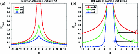
, where , , . always works well in terms of extending and smoothing gradient vector. Generally, the factor plays a role analogous to scale space filtering, the greater the value of , the greater the smoothing effect on the results. This property suggests that GVC would be robust to noise. In addition, large makes the potential to degrade fast with distance and vice versa. Thereby it allows the GVC snake to preserve edges and to drive into C-shape concavities.Fig. 3
Analysis of the behavior of  and
and  in 1D case
and in 1D caseIn order to well understand the behavior of  and
and  , we plot the proposed kernel
  in 1D case with different
  and
and  in Fig. 3. It can be seen from Fig. 3a that, the larger the value of
  , the smaller the value of
  at points nearby
  , but almost unchanged at points far from
  . Note that
  is not defined at
  when
when  , we set
  for the sake of exhibition. Similar strategy is employed in Fig. 3b. From Fig. 3b, we can observe that the larger the value of
  , the faster
  degrades with distance. For example, although point A is
  while B is
  far from
  , due to varying
  , the values of
  at point A and B are almost identical. It seems as if the point B is as near as A to
  in terms of the value of
  . Similar results can be observed for points C and D and it seems as if the point C is as far as D from
  . As a result, if one wants to separate two closely-neighbored objects or preserve edges, one can use large
  such that nearby points are less weighed as if they are far away. On the other hand, if concavity is too deep, small
  can be employed to weigh relatively more on faraway points as if they are nearby.
and , we plot the proposed kernel in 1D case with different and in Fig. 3. It can be seen from Fig. 3a that, the larger the value of , the smaller the value of at points nearby , but almost unchanged at points far from . Note that is not defined at when , we set for the sake of exhibition. Similar strategy is employed in Fig. 3b. From Fig. 3b, we can observe that the larger the value of , the faster degrades with distance. For example, although point A is while B is far from , due to varying , the values of at point A and B are almost identical. It seems as if the point B is as near as A to in terms of the value of . Similar results can be observed for points C and D and it seems as if the point C is as far as D from . As a result, if one wants to separate two closely-neighbored objects or preserve edges, one can use large such that nearby points are less weighed as if they are far away. On the other hand, if concavity is too deep, small can be employed to weigh relatively more on faraway points as if they are nearby.