Chapter 2
T2 Contrast
Scott M. Duncan and Timothy J. Amrhein
CASE 1
1. What type of sequence is this? How do you know?
2. What TR and TE parameters would you use to obtain T2 weighting with a spin echo sequence?
3. What tissues have long T2 relaxation times? Do they appear bright or dark on T2-weighted images?
4. What is the normal maximal diameter for the central canal?
ANSWERS
CASE 1
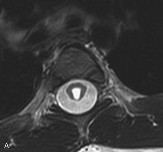
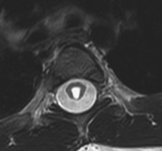
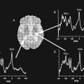
FIGURE 1A. Axial T2-weighted image of the thoracic spine demonstrates a large T2-hyperintense space involving the central canal and surrounding white matter.
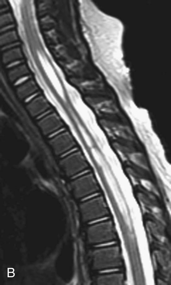
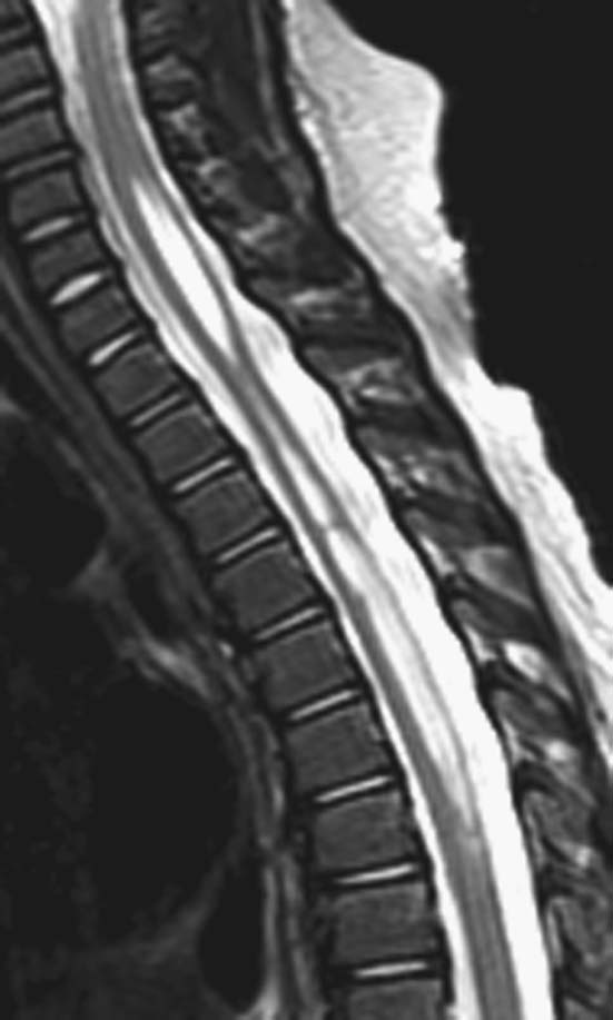
FIGURE 1B. Sagittal T2-weighted image of the thoracic spine. Vertically oriented central hyperintensity extends throughout the cervical and thoracic cord.
1. These are T2-weighted sequences. This can be discerned because structures composed predominantly of water are bright (hyperintense) on T2-weighted sequences. Such structures include the cerebrospinal fluid in brain and spine images, the gallbladder or fluid in the abdomen, the bladder in the pelvis, and intra-articular synovial fluid in the extremities.
2. To achieve T2 weighting on a spin echo image, one would use a long time to repetition (TR) and an intermediate to long time to echo (TE).
3. Tissues that contain mostly water have long T2 relaxation times and they appear hyperintense (bright) on T2-weighted images. This is in contrast to tissues with long T1 relaxation times, which appear dark on T1-weighted sequences.
4. In adults, the central canal is often not identified as it is below the resolution of the scan. A canal diameter greater than 3 mm is considered to be abnormal.
Diagnosis:
Syringohydromyelia.
Part 1: Basic Spin Principles and T2 Relaxation
After a radiofrequency (RF) pulse tips the net (or main) magnetization into the transverse plane, it will gradually lose phase coherence as individual protons will experience a dephasing process as a result of spin-spin interactions. This phenomenon is known as T2 or transverse relaxation (or decay). At the same time, the magnetization will also return to its original state via T1 or longitudinal relaxation (or recovery). This chapter focuses on the T2 or transverse relaxation.
An RF pulse generates a magnetic field oriented in the transverse (or xy) dimension. During its application, the net magnetization along the longitudinal direction will be tipped into the transverse plane. Immediately after this rotation, all protons naturally would have the same phase and thus phase coherence.1 Once the RF pulse is turned off, there is progressive loss of phase coherence. This occurs because individual protons begin to precess at slightly different frequencies due to different local microenvironments and spin-spin interactions. The resultant slight differences in precession frequencies among protons causes phase dispersion, signal cancellation, and loss of transverse magnetization. It is important to note that transverse relaxation or decay is therefore due to loss of order (i.e., phase dispersion) rather than the loss of magnetization.
Why does this phase dispersion occur if all of the hydrogen protons are exposed to the same external magnetic field? It occurs because there are inherent inhomogeneities within the magnetic field that lead to differing magnetic microenvironments and subsequently slightly different proton precession frequencies. There are two separate causes of magnetic field inhomogeneity: inhomogeneities within the external magnetic field (T2’) and microscopic interactions between adjacent protons (T2). The combined loss of signal resulting from both of these causes is called T2* decay. The dephasing effects from the external magnetic field have a much larger contribution to T2* decay than do the T2 effects. Unfortunately, inhomogeneities that arise from the external magnetic field are independent of the patient and therefore provide little information about the patient. Fortunately, the loss of phase coherence from these static inhomogeneities can be reversed, for example, by a 180° refocusing pulse. (This point will become more important when we discuss spin echo imaging.) Loss of phase coherence arising from T2 effects is not reversible but does provide information about the microenvironment that the proton is experiencing, aiding in tissue characterization.
Let’s further explore the concept of T2*. A magnetic resonance (MR) signal can only be detected when the magnetization is in the transverse plane. When an RF pulse is applied, the magnetization vector is “tipped” into the transverse plane while still rotating about the z-axis at the Larmor frequency. The resultant MR signal appears as a sinusoidal wave, peaking when the vector is pointed toward the detector and reaching a trough when the vector is pointed 180° away from the detector. Further, remember that immediately after the RF pulse is turned off, phase dispersion occurs, causing a rapid and continuous fall in signal. The resultant waveform, called free induction decay (FID), is a combination of this declining magnetization and the 360° rotating signal. As shown in Figure 1, the FID appears as an oscillating waveform that rapidly falls to zero. The FID describes the detected MR signal, which experiences a rapid exponential loss at the rate of T2*.
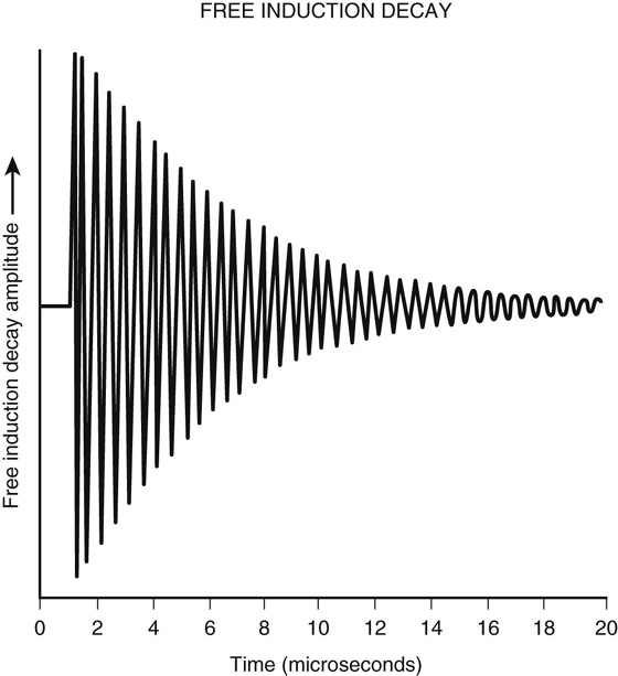
FIGURE 1. Free induction decay.
The component of T2* that does provide information about the patient is the T2 relaxation. T2 relaxation occurs at an exponential rate analogous to T2* relaxation, except at the rate of T2. As mentioned previously, the T2 relaxation time is governed by individual protons’ local environment and spin-spin interactions, resulting in phase dispersion. In general, all molecules are influenced by their local magnetic microenvironment, which fluctuates over time. Larger molecules have relatively slowly varying magnetic fields. As a result, this more static magnetic field variation results in some areas with stronger local magnetic fields and other areas with weaker local magnetic fields. These differences result in different precessing frequencies among the protons, causing significant dephasing. Smaller molecules (such as water), in contrast, are rapidly moving, leading to an averaging of the magnetic field variability (i.e., the smaller molecules experience a mixture of both stronger and weaker magnetic fields that is averaged out over time). This leads to increased homogeneity of the experienced magnetic field, resulting in less phase dispersion and therefore longer T2 relaxation times. Unlike T1 relaxation times, T2 relaxation times are less dependent on magnetic field strength. T2 relaxation times for most tissues within the body range from 30 to 60 msec. The T2 relaxation time for cerebrospinal fluid, which is mostly free water, is 1000 msec.
T2-weighted (T2W) images are well suited for the detection and assessment of most pathologic processes, as pathology often results in increased water content, causing T2 hyperintensity relative to the isointense signal of normal soft tissue.
Part II: T2 Contrast and Pulse Sequence Considerations
Two general categories of sequences are employed to produce images weighted by transverse relaxation times: spin echo (SE) sequences and gradient-recalled echo (GRE) sequences. Pure T2W images can only be obtained with SE sequences. GRE sequences can produce T2*-weighted images, but are unable to produce purely T2W images for reasons that will be explained later.
SE imaging involves an initial 90° RF pulse that tips the longitudinal magnetization into the transverse plane and aligns the phases. This is then followed by a 180° pulse that realigns the spins. Remember, when the initial 90° RF pulse is turned off, the protons immediately begin to dephase. Subsequently, a 180° RF pulse (also known as a “refocusing pulse”) is used to reverse the precession direction of the protons (i.e., instead of rotating clockwise, they begin to rotate counterclockwise about the z-axis or vice versa). This has the intended effect of reversing the phase dispersion caused by static magnetic field inhomogeneities. The reversal occurs because the protons continue to precess at the same rate that they did in developing different phases; however, they now do so in the reverse direction. Thus, over the same amount of elapsed time a faster precessing proton that was able to change phase in relation to its slower precessing counterparts now precesses faster than the slower proton, but in the opposite direction, and effectively “catches back up” with the slower precessing proton. By this process, the transverse magnetization that was lost due to magnetic field inhomogeneities will be recovered (Figure 2). Therefore, any loss of signal in an SE sequence is from phase dispersion due to microscopic fluctuations in the magnetic field caused by the local molecules (i.e., pure T2 relaxation).
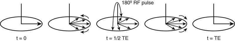
FIGURE 2. Effect of 180° refocusing pulse on phase dispersion. Once the initial 90° RF pulse is turned off, the protons begin to dephase. The 180° refocusing pulse reverses the phase dispersion and results in rephasing of the protons, which occurs maximally at TE (= 2τ in this figure). Adapted from Clare S: Principles of magnetic resonance imaging. In Functional MRI: Methods and Applications. Doctor of Philosophy Thesis, October 1997, University of Nottingham, UK. Available at http://users.fmrib.ox.ac.uk/~stuart/thesis/chapter_2/section2_4.html.
In SE sequences, there are two main parameters that affect the “weighting” of an image (i.e., T1, T2, or proton density weighting): the time to repetition (TR) and the time to echo (TE). In generating an image, the protons within a patient are repeatedly exposed to RF pulses in order to fill each line of K-space. During the first excitation, all of the longitudinal magnetization is “tipped” into the transverse plane. Over time, the longitudinal magnetization returns (or recovers) at a tissue-specific rate, which is based on its T1 relaxation time. If the TR is shorter than the time it takes to fully recover longitudinal magnetization (i.e., another 90° RF pulse is introduced prior to complete longitudinal magnetization recovery), then there will be less signal available to “tip” into the transverse plane with the next pulse. Given a short TR, substances with short T1 relaxation times will recover more longitudinal magnetization and will therefore appear hyperintense (bright), whereas substances with long T1 relaxation times will not recover signal prior to the next excitation pulse and will be hypointense (dark). In contradistinction, if the TR is long, then both tissues will fully recover their longitudinal relaxation and the T1 relaxation time will not significantly affect the final signal.
The TE is defined as the time between the first 90° RF pulse and the time of signal acquisition. As was previously described, SE sequences employ a 180° pulse to realign dephased spins and remove signal loss from magnetic field inhomogeneities. To acquire maximal signal in an SE image, the 180° RF pulse is placed at one half of the TE. In other words, the spins that dephase during the first half of the TE are subsequently rephased during the second half of the TE, which results in maximal signal at the time of signal acquisition. All signal loss is therefore secondary to the inherent T2 relaxation of the tissue (fluctuations in the local magnetic field secondary to the structures of the local molecules). An intermediate to long TE allows enough time for tissues with short T2 relaxation times to lose some signal (and appear hypointense), while tissues with long T2 relaxation times still retain most of their signal (and appear hyperintense). However, if the programmed TE is very short, not enough time will have elapsed to allow for any significant T2-related decay and no tissue will experience any significant transverse decay; therefore, there will be no contrast between different types of tissues.
As you can see from the description above, manipulation of the TR provides separation of tissues based on their T1 relaxation times and changing the TE results in tissue separation based on inherent T2 relaxation properties. The TE and TR can therefore be adjusted to maximize signal based upon either the T1 or the T2 relaxation properties of a tissue. This preferential bias toward one relaxation parameter versus another is referred to as “weighting.” With T2W images, one minimizes the T1 relaxation effects on signal production by lengthening the TR, and maximizes the T2 relaxation effects by choosing an intermediate to long TE. As a memory aid, one might consider that T“1” is a smaller number than T“2”and thus has smaller TRs and TEs. For a typical T2W image, the TR is greater than 2000 msec and the TE is greater than 100 msec.
GRE sequences involve a single “excitation” RF pulse that transfers some of the longitudinal magnetization into the transverse plane, where it can be used to acquire signal. A significant difference between GRE sequences and standard SE sequences is the absence of a 180° refocusing pulse. Without this additional pulse, the phase dispersion caused by inhomogeneities in the main magnetic field is not corrected. Therefore, the loss of signal in a GRE sequence is due to T2* effects. As was previously described, these T2* effects are significantly influenced by the inhomogeneity in the external magnetic field and do not provide exclusive information about the relaxation properties of the tissue being imaged.
Recently, steady-state GRE sequences have been used that produce more weight on T2 and not T2* contrast. In steady-state imaging, both the longitudinal and transverse magnetization enter a steady state. In spoiled gradient imaging, the residual transverse magnetization after the echo has been recorded is usually spoiled by use of a spoiler gradient before the next TR. However, in steady-state imaging, the residual transverse magnetization is added back to the longitudinal magnetization, resulting in higher signal to noise ratio. The amount of residual transverse magnetization is based on the T2 time. Substances with long T2 times will have more residual magnetization to add back to the longitudinal magnetization, which can be used in subsequent excitations. Additionally, molecules with short T1 times will have recovered more longitudinal magnetization before the next TR, resulting in more magnetization in subsequent excitations. Thus, the steady-state sequences are T2/T1 weighted. In other words, substances that have long T2 times (water) and short T1 times (fat) will be bright on these sequences.1 These sequences are commonly used in cardiac imaging and in imaging the base of the skull, where high-resolution thin-slice T2W images are used. Further discussion about steady-state imaging and its role in cardiac imaging is provided in Chapter 10.
CASE 2
FIGURE 2A. Axial T2W fast spin echo (FSE) image of the abdomen: normal, with bright fat signal.
FIGURE 2B. Axial T2W FSE image with fat saturation of the abdomen: normal, with dark fat signal.
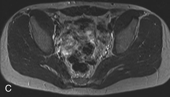
FIGURE 2C. Axial T2W SE image of the pelvis: normal, with intermediate gray signal of fat.
Diagnosis:
Normal fat appearance on FSE, fat saturation (fat-sat) FSE, and SE sequences.
Physics Discussion
As was mentioned in the beginning of the chapter, T2W images have a relatively long TR to allow the longitudinal magnetization to recover. In order to shorten the total scan time, multiple 180° refocusing pulses can be applied (and thus multiple echoes collected) during a single TR interval. The number of refocusing pulses applied during a single TR interval is called the echo train length or turbo factor. Imaging time reduction is directly proportional to the echo train length (i.e., for an echo train length of 9, the imaging time is reduced by a factor of 9). These sequences are known as turbo or fast spin echo (FSE) sequences. The number of additional echoes depends on the length of the TR. Sequences with longer TRs, such as T2W images, can fit 8 or more TEs into each TR. Blurring occurs in sequences with short TEs, such as T1-weighted (T1W) and proton density images, so only a short echo train length of 3 to 7 can be used. Because of its much improved image time, the FSE technique has completely replaced conventional SE imaging for T2W imaging. In fact, most residents and young attendings have never seen an SE T2W imaging sequence in clinical practice.
The FSE sequences allow T2W images of the abdomen to be obtained in a single breath hold. This is not possible with the SE technique and is why the SE image shown in Case 2 is of the pelvis. Imaging the abdomen with an SE sequence would have resulted in blurring secondary to respiratory motion artifact unless a respiratory triggering or gating method is applied.
One consequence of the FSE technique is the relatively increased signal intensity of fat in comparison with a conventional SE image (this is one reason why T2W sequences are often fat-saturated or inversion recovery sequences). As you may recall, fat has a relatively short T2 relaxation time secondary to its large molecular size, which results in rapid loss of transverse magnetization. Further, fat molecules are subject to signal loss secondary to a phenomenon called J-coupling, which is a very complex topic and applies more to nuclear magnetic resonance spectroscopy than to MR imaging. Macromolecules, such as lipids, share electrons between their nuclei via the electron cloud, causing a slight alteration in the local magnetic fields of different nuclei on the same molecule. This, in turn, results in a change in the precessional frequencies of these different nuclei leading to a rapid dephasing that occurs in addition to the normal T2 dephasing. This phenomenon is referred to as J-coupling and explains why fat appears with low to intermediate signal on T2W SE sequences. Why, then, does fat appear brighter when using FSE techniques? The answer lies in the multiple refocusing pulses employed in an FSE sequence, which do not allow sufficient time for J-coupling dephasing to occur. This prolongs the overall T2 relaxation of fat and leads to the relatively higher signal of the fat on the FSE T2W image in comparison with the conventional SE T2W image.
CASES 3, 4, AND 5: COMPANION CASES
Case 3
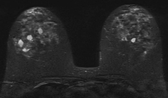
FIGURE 3. Axial T2W FSE image with fat saturation (fat-sat): multiple bilateral T2-hyperintense lesions within the breasts consistent with simple cysts.
Diagnosis:
Multiple bilateral simple breast cysts.
Discussion:
The criteria for diagnosing a simple cyst within the breast on magnetic resonance imaging (MRI) are similar to those in ultrasound. The cyst is usually homogeneously hyperintense (fluid bright) on a T2W image and should demonstrate a smooth contour. On a T1W image, the cyst is usually uniformly hypointense and should exhibit no internal enhancement after the administration of contrast. A thin rim of peripheral enhancement is acceptable.2,3
Case 4
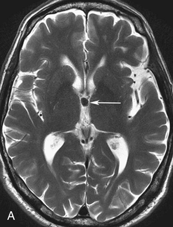
FIGURE 4A. Axial T2W image. A small homogeneous T2-hypointense mass is seen in the region of the foramen of Monro (arrow).
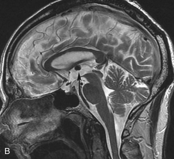
FIGURE 4B. Sagittal T2W image. The T2-hypointense mass is redemonstrated in the region of the foramen of Monro (arrow).
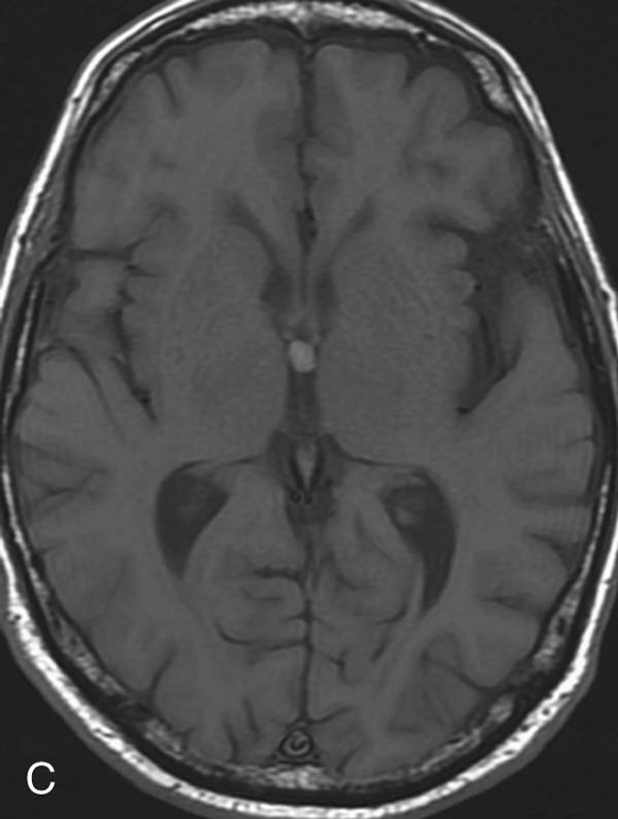
FIGURE 4C. Axial T1W image. The mass exhibits T1 hyperintensity.
Diagnosis:
Colloid cyst.
Discussion:
There are many different appearances of cysts on MRI. Colloid cysts are typically T2 hyperintense. However, in this case the concentration of internal protein and paramagnetic material is high, which results in T2 hypointensity and T1 hyperintensity. Colloid cysts have a very characteristic location at the foramen of Monro, which greatly aids in their diagnosis.4 As with other cysts, colloid cysts should be homogeneous and should not exhibit central enhancement.
Case 5
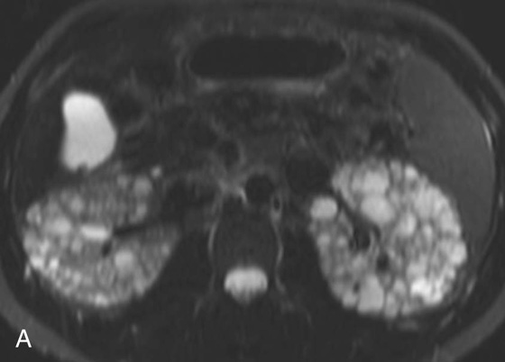
FIGURE 5A. Axial T2W fat-sat FSE image.
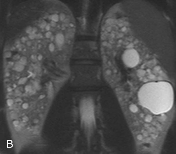
FIGURE 5B.
Related posts:

Stay updated, free articles. Join our Telegram channel

Full access? Get Clinical Tree


