Contrast

Chapter 1

T1 Contrast

Phil B. Hoang, Manjiri M. Didolkar, Allen W. Song, and Elmar M. Merkle

CASE 1

1. What weighting are these images?

2. Which parameter gives the most T1 weighting on a spin echo sequence, a long or short TR?

3. Do tissues that produce high signal on T1-weighted images have a long or short T1 relaxation time?

4. Where do you normally expect to find the neurohypophysis?

5. The patient presented with short stature; what is the diagnosis?

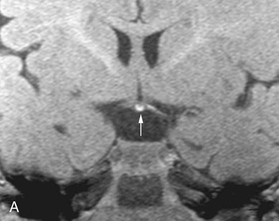
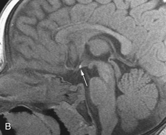
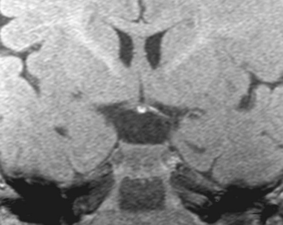
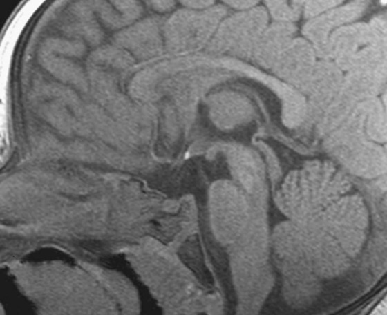
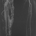
FIGURES 1A AND 1B. Coronal (A) and sagittal (B) T1-weighted images of the brain. Small high T1 signal focus at the superior aspect of the infundibulum (arrows) is demonstrated. Lack of the expected “bright spot” of the neurohypophysis within the posterior sella is observed on the sagittal image (B).

1. These are T1-weighted images.

2. A short time to repetition (TR) (400 to 800 msec) on a spin echo pulse sequence gives you T1 weighting.

3. Tissues that produce high signal on a T1-weighted image (such as fat) exhibit a short T1 relaxation time.

4. The neurohypophysis is normally located in the posterior sella.

5. Ectopic neurohypophysis.

Discussion

The normal T1 “bright spot” of the neurohypophysis is due to the proteins bound to vasopressin. Absence of the bright spot in its expected position or location within the posterior sella is consistent with ectopic neurohypophysis, a cause of short stature in children. The diagnosis is made by recognizing the abnormal position of the neurohypophysis on a T1-weighted (T1W) image, which in this case was in the superior aspect of the infundibulum.

Part I: Basic Spin Principles and T1 Relaxation

Because of its abundance in the human body, hydrogen is the most frequently imaged nucleus in clinical magnetic resonance imaging (MRI). Hydrogen has a considerable angular magnetic moment, with its single, positively-charged proton acting as a tiny, spinning bar magnet. Protons normally spin in random directions in the absence of an external magnetic field; because of this random movement, the magnetic vector sum of these protons is typically zero.

When placed in a strong external magnetic field (B0), these protons align either parallel (low energy) or antiparallel (high energy) with respect to B0; more protons tend to align parallel to B0 since less energy is required to do so. Because they possess both magnetic and angular momentum, the protons precess, or wobble, around the axis of B0 instead of spinning in a tight circle; this precession motion confers both longitudinal (Mz) and transverse (Mxy) components in the magnetic moments of the protons. Protons tend to precess at a certain frequency while under the influence of B0, which is called the Larmor frequency. The Larmor frequency defines the frequency at which the radiofrequency (RF) pulse is broadcast to induce proton resonance, or excitation. The Larmor frequency is proportional to the strength of the main magnetic field; at 1.5 Tesla, the Larmor frequency of hydrogen protons is 63.8 MHz, and it is approximately 127 MHz at 3 Tesla.

The vector sum of the magnetic moments of the precessing protons (Mz and Mxy) results in a net equilibrium magnetization (M0). This magnetization vector is primarily in the longitudinal direction (Mz) since more protons align in parallel with B0. The transverse component (Mxy) does not contribute significantly to M0, as the protons do not spin in phase with each other and effectively cancel each other out. As the energy of B0 increases, so does the energy differential between protons in the low (parallel) and high (antiparallel) states, with increasing numbers of protons aligning parallel to B0. This results in a significant directional (vector) component of the net magnetization. However, the receiver coil, which is the component of the MRI machine that detects signals, is sensitive only to variations of the magnetization vector; the original main magnetization along the z direction, even though it is precessing, is viewed as a “stationary” vector from the receiver coil perspective. Given this, something must be done to perturb the system and generate detectable signal changes that can be picked up by the receiver coils; this comes in the form of an RF excitation pulse.

Application of the RF pulse (a short burst of electromagnetic energy) results in energy absorption by protons. In order for this energy transfer to occur, the RF pulse and precessing protons must have the same frequency. This results in a change in the energy level of the protons, which go from the low-energy (parallel) state into the high-energy (antiparallel) state. Simultaneously, there is a gain in the protons’ phase coherence, as the protons receive their initial phase that is synchronized. This produces a net loss of longitudinal magnetization and a net gain in transverse magnetization, respectively. Conceptually speaking, this is better known as the “tipping” of net magnetization vector from the longitudinal axis (Bz) into the transverse plane (Bxy), such that the precession motion can be visible and signal changes detectable by the receiver coils. The degree of transverse magnetization generated depends on both the amplitude of the RF pulse and length of time it is administered; complete rotation of protons into the transverse plane is the result of a 90° RF pulse.

After cessation of the excitation pulse, the resonating protons “relax” back into their equilibrium state, which occurs by two mechanisms: transverse (T2) and longitudinal (T1) relaxation. While these two mechanisms occur concurrently, they do so at different rates. Briefly, transverse relaxation refers to loss of phase coherence due to interactions between spinning protons (spin-spin). This leads to a net decrease in transverse magnetization, and is also referred to as T2 decay. This concept is discussed in greater detail in Chapter 2.

In T1 relaxation, the resonating proton returns to its thermal equilibrium state by transferring energy to the other nuclei in its surrounding, or lattice. This mechanism is commonly referred to as spin-lattice relaxation, and results in a net increase in longitudinal magnetization. T1 relaxation occurs at an exponential rate; at time T1, longitudinal magnetization has returned to 63% of its final value, and at time 3*T1, longitudinal magnetization has returned to 95% of its final value. The differences in tissue T1 relaxation are responsible for the contrast on a T1W image and depend on the efficiency of energy transfer from proton to lattice. Tissues with short T1 relaxation times (fat) generate high signal, while tissues with long T1 relaxation times (water) generate low signal.

Differences in T1 relaxation are primarily attributed to the natural movement unique to a molecule. In short, the more similar the molecule’s natural motional frequency is to that of the Larmor frequency, the more efficiently energy transfer to its lattice occurs. This results in a short T1 relaxation time. Small molecules, such as those found in free water (cerebrospinal fluid), move rapidly; on the other side of the spectrum, macromolecules such as protein move at a slower pace. While the motional frequencies of these molecules differ immensely, both exhibit long T1 relaxation times because both move at a frequency much different than the Larmor frequency. Intermediate-sized molecules, such as fat, move at frequencies very similar to the Larmor frequency and thus exhibit short T1 relaxation times.

The term T1 shortening refers to a decrease in the T1 relaxation time of a tissue, leading to greater signal intensity on a T1W pulse sequence than is expected. This change is usually under the influence of agents that induce T1 relaxivity of nearby free water protons. The mechanisms exhibited by these agents include paramagnetic (gadolinium, manganese, methemoglobin) or hydration layer (proteins, ionic calcium) effects. The most commonly known paramagnetic agents are the gadolinium chelates used in contrast-enhanced sequences; these agents, as well as the mechanisms of T1 relaxivity exhibited by these agents, are discussed in greater detail in Chapter 4.

Part II: T1 Contrast and Pulse Sequence Considerations

An important point to consider when interpreting any magnetic resonance (MR) image is that image contrast is not exclusively due to differences in T1, T2, or proton density; these contrasts all make some contribution. However, by manipulating certain operator-dependent parameters, we can have more of one contrast and less of the others.This is why we use the terms T1, T2, and proton density weighting when describing the contrast in an image.

Spin Echo

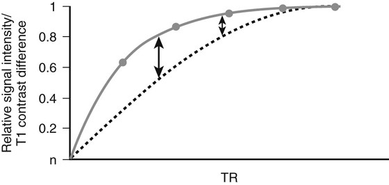
In a conventional spin echo (SE) sequence, the 90° RF pulse is followed by a 180° refocusing pulse, which is administered at the halfway point of the echo time and is used to bring the protons back into an in-phase (i.e., synchronized) state. The parameter with the greatest effect on T1 contrast on a conventional SE sequence is the time to repetition (TR), which is the time interval between successive excitation pulses. A moderate TR can be determined to optimize the T1 contrast. The TRs for T1W SE sequences are typically in the range of 400 to 800 msec. As the TR lengthens, most tissues recover their longitudinal magnetization and produce signal; while this will increase overall signal-to-noise ratio in the image, it will diminish T1 contrast (Fig. 1).

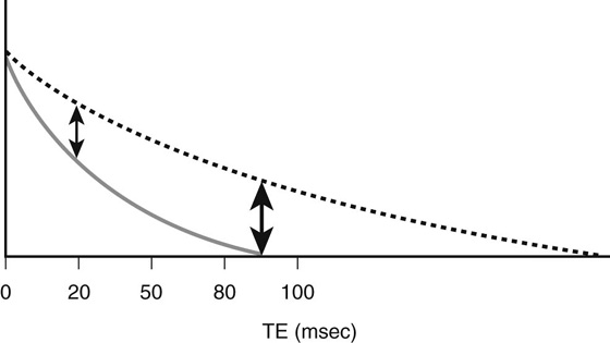
FIGURE 1. Following the excitation pulse, tissues regain longitudinal magnetization (Mz) at rates determined by their specific T1 relaxation time. A short TR maximizes differences in T1 contrast (large arrow). A longer TR minimizes T1 contrast.

While modifying TR can optimize T1 contrast, adjusting the length of the second parameter, the time to echo (TE), governs T2 contrast. The TE is the time interval between the excitation pulse and signal collection; this parameter has the greatest effect on decreasing the contribution from T2 contrast (Fig. 2). To minimize the T2 contrast (so that T1 contrast is dominant), the TE should be kept as short as possible (15 to 25 msec). A moderate TE would generate significant T2 contrast (see Fig. 2).

FIGURE 2. Mxy decay (transverse magnetization). By using a short TE (~20 msec), differences in T2 contrast in the image are minimized. These differences in T2 contrast would be more significant if a longer TE (~100 msec) were used.

Gradient-Recalled Echo (GRE)

This class of pulse sequences uses an excitation pulse with a variable “flip” angle (< 90°) and rephases protons with gradients of equal magnitude and duration but opposite polarities. This is opposed to conventional SE sequences, which apply a 180° refocusing pulse to rephase protons. In GRE acquisitions, the flip angle often plays a role in changing T1 contrast. Small flip angles allow the longitudinal magnetization to recover more rapidly. As such, the TRs used are typically short (< 200 msec), as are the TEs (< 10 msec to minimize T2 contrast).

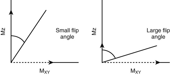
T1 weighting in GRE sequences is maximized by using an excitation pulse with a large (~ 50° to 80°) flip angle, a short TR (~ 100 msec), and a short TE (< 10 msec). Both the flip angle and the TR have the greatest influence on T1 weighting, with the effect of the flip angle illustrated in Figure 3. Using large flip angles places an emphasis on T1 contrast as signal intensity produced depends on tissue specific T1 relaxation times. With small flip angles, different tissues retain most of their longitudinal magnetization (Fig. 3, solid arrows); because of this, the longitudinal magnetizations of tissues (and thus signal intensity) are similar on a T1W sequence, which reduces T1 contrast (see Fig. 3).

FIGURE 3. A larger flip angle “tips” most of the protons into the transverse plane (dashed arrow) with a small amount of longitudinal magnetization remaining. Similar to SE sequences, the signal differences between tissues are then dependent on tissue-specific T1 relaxation times.

Strengths of GRE sequence over conventional SE include faster image acquisition (due to shorter TRs) and decreased RF power deposition (due to the lack of a 180° refocusing pulse). In exchange, signal is sacrificed; GRE suffers from irretrievable signal loss due to magnetic field inhomogeneities and susceptibility effects (T2*) because it does not apply a refocusing pulse. Thus, GRE sequences are generally lower in signal-to-noise ratio compared to SE sequences.

An important consequence of the short TRs used in GRE is the residual transverse magnetization remaining prior to the next excitation pulse. If left alone, the transverse magnetization will contribute to the longitudinal component after the next excitation pulse is administered, which eventually alters image contrast. To resolve this issue, a spoiler mechanism is used prior to the start of the next TR to prevent buildup of a transverse magnetization steady state and makes the magnetization in the longitudinal direction the chief contributor to Mz at the next excitation pulse.

When extremely short acquisition times are needed, “ultrafast” GRE sequences are used. These sequences acquire images in 1 second or less by using extremely short TRs (< 3 msec) and small flip angles. Since these parameters are generally unfavorable for the T1 weighting needed in contrast-enhanced sequences, an additional step is needed to boost T1 contrast. A preparatory pulse applied prior to the excitation pulse inverts the longitudinal magnetization, which introduces T1 weighting by emphasizing differences in tissue T1 relaxation; this concept is discussed further in Chapter 6.

Part III: Clinical Applications

The contrast of a T1W sequence provides an important overview of anatomy. The two tissues that produce the most predictable signal intensity on a T1W image are fat and free water. This is a reflection of each tissue’s T1 relaxation time, which is short for fat (~250 msec at 1.5T) and long for water (~2500 msec at 1.5T). Normal solid organs (brain, muscle, liver, spleen, kidneys) have intermediate relaxation times, ranging from 490 msec (liver) to 970 msec (gray matter) at 1.5 Tesla (1.5T). The differences in T1 contrast are secondary to the varying ratios of extracellular water and macromolecules. For example, the normal pancreas produces the greatest signal intensity on a T1W image of the solid abdominal organs due to its high protein synthesis and intracellular paramagnetic agents. Bone marrow demonstrates variable signal intensity depending on its ratio of red-to-yellow marrow.

CASES 2 AND 3: COMPANION CASES

Case 2

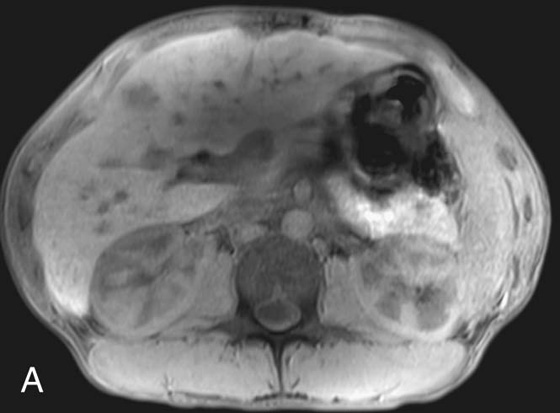
FIGURE 2A. Axial T1W image of the upper abdomen with fat suppression. An ill-defined low T1 signal lesion is seen in the anterior right hepatic lobe.

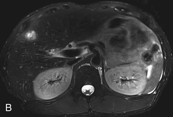
FIGURE 2B. Axial T2-weighted (T2W) image with fat suppression. The lesion is predominantly high in T2 signal; perilesional high T2 signal extends peripherally from the lesion.

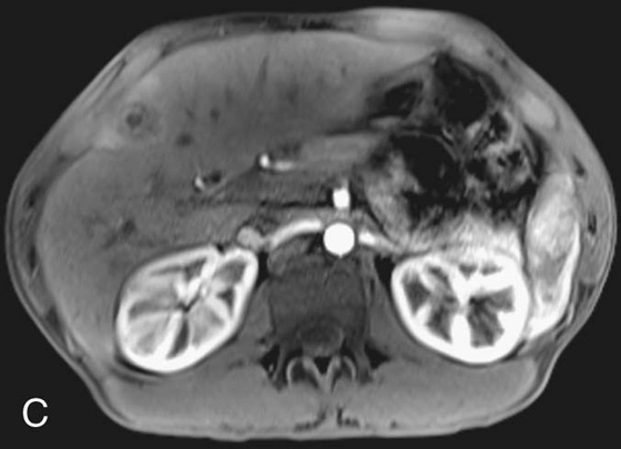
FIGURE 2C. Axial postcontrast T1W image. The lesion demonstrates peripheral rim enhancement; there is parenchymal enhancement surrounding the focus, consistent with hyperemia or edema.

Only gold members can continue reading. Log In or Register to continue