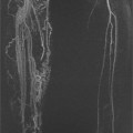
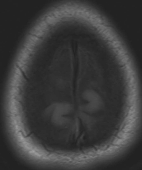
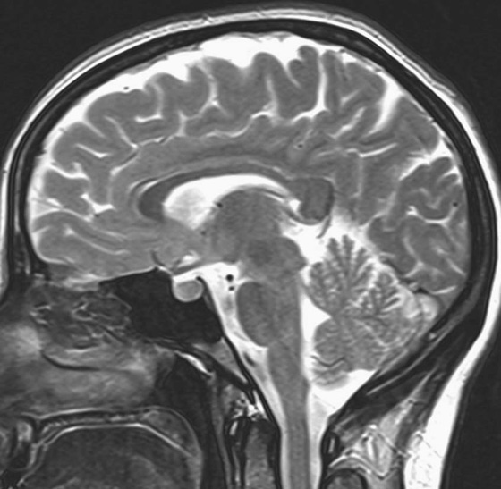
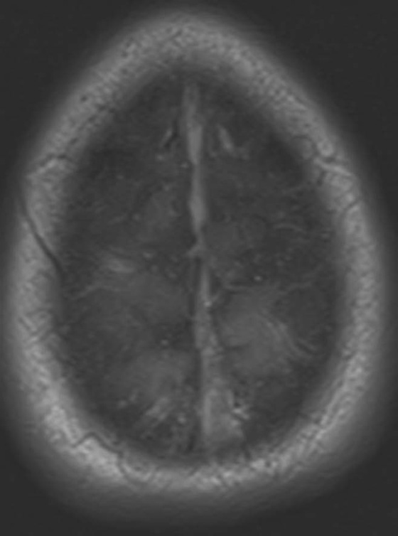
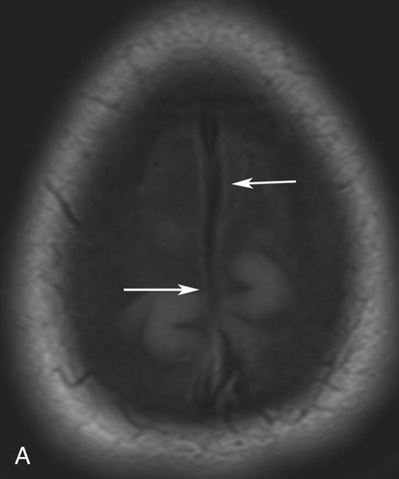
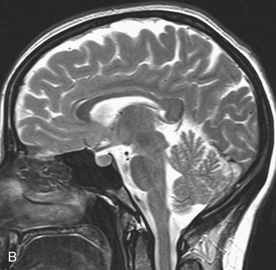
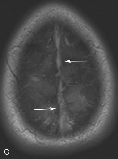
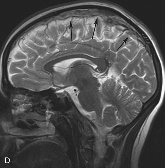
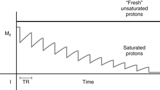
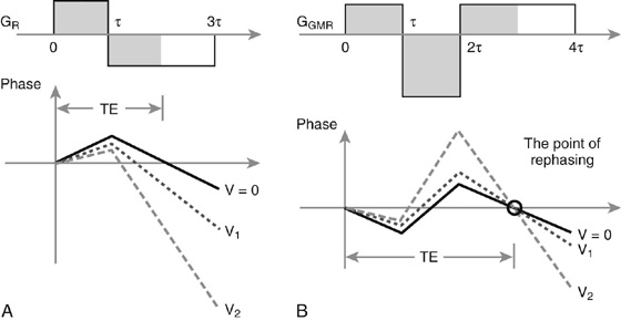
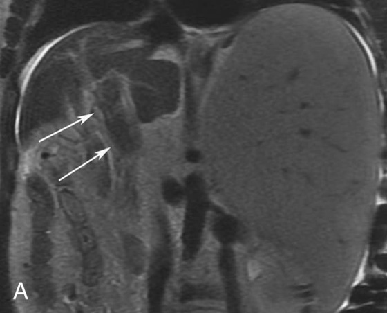
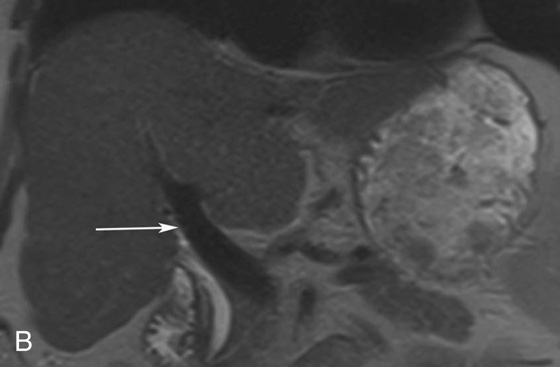
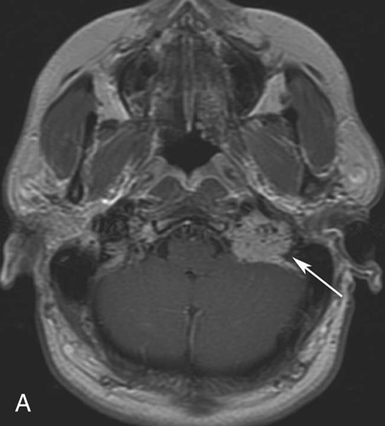
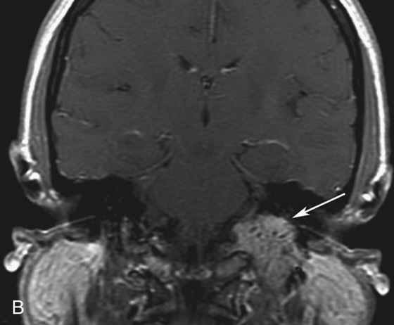
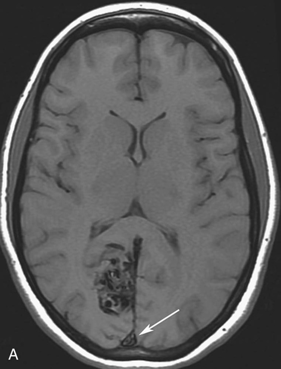
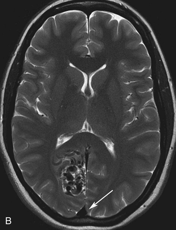
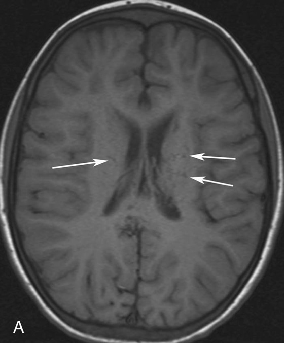
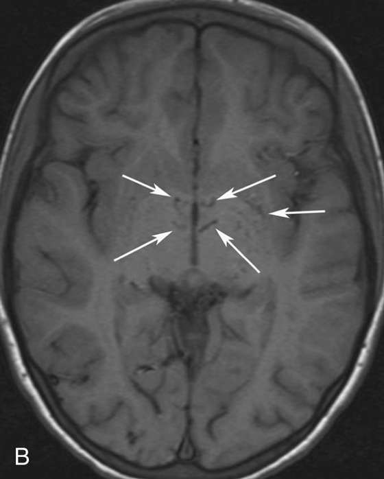
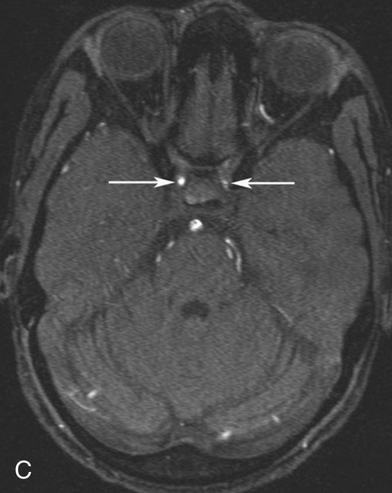
FIGURE 1A. Axial T1-weighted fast spin echo (FSE) image demonstrates a flow void (arrows) in a patent superior sagittal sinus.

FIGURE 1B. Sagittal T2-weighted FSE image redemonstrates the thin flow void in the superior sagittal sinus.

FIGURE 1C. Axial T1-weighted FSE image, demonstrates expansion and signal within the superior sagittal sinus and the lack of a flow void (arrows).

FIGURE 1D. Sagittal T2-weighted FSE image redemonstrates the expansion of and signal within the superior sagittal sinus (arrows).

The answer is actually quite simple. Spin echo techniques result in flow voids, while gradient-recalled echo techniques result in flow-related enhancement. These are, of course, generalizations and there are exceptions to this rule (we will explore these later). However, in the majority of cases this simple generalization holds true.

Cardiac MRI takes advantage of the distinct flow-related properties of these two magnetic resonance (MR) sequences to image the cardiovascular system. The generic descriptors “black blood” technique and “white blood” technique are the result of flow voids and flow-related enhancement, respectively. In other words, blood is dark in the “black blood” technique primarily as a result of the flow void phenomenon produced by a spin echo sequence. Conversely, blood is bright in the “white blood” technique, based on the flow-related enhancement found in a gradient-recalled echo sequence.

Flow voids and flow-related enhancement are both based on the same “time-of-flight” phenomenon. The basis of this phenomenon is that flowing protons within blood do not experience the same radiofrequency (RF) pulses and magnetization as that of stationary protons. Thus, the signal obtained from flowing protons is different than that from stationary protons.

Let’s begin with a discussion of spin echo imaging. Spin echo imaging uses two RF pulses to produce a signal. The first is a 90° pulse that tips the longitudinal magnetization into the transverse plane. Subsequently, a 180° pulse realigns the dephased spins in order to produce an echo. The proton must experience both RF pulses to create a signal. For example, if a moving proton is hit with the initial 90° RF pulse and then moves out of the imaging plane before the 180° RF pulse (thereby avoiding the 180° pulse), the dephased protons will not be refocused. This absence of refocusing means that all of the transverse magnetization will remain dephased and no signal will be obtained. Alternatively, if the proton is outside of the imaging slice when the 90° pulse is applied, but then moves into the slice when the 180° pulse is applied, the proton’s magnetization will be flipped 180° (reversed or “upside down”) in the longitudinal direction. In this scenario, there will be no transverse magnetization to provide a signal (as the initial 90° RF pulse was missed). In both of the provided scenarios, the result is absence of signal, or a flow void.

While we may think of a flow void as a complete loss of signal, there is, in reality, a spectrum ranging from full normal signal to a complete signal void. The amount of signal void is dependent upon the velocity of the proton, the slice thickness, the time to echo (TE), and the course of the vessel. The greater the velocity of the proton, the quicker it will move out of the imaging slice and the less time it has to experience both the 90° and 180° RF pulses. Thinner slices mean that there are shorter required distances to traverse the imaging slice, thus less time to experience both RF pulses (and a greater likelihood of a flow void). Longer TEs mean that there is more time between the 90° and 180° RF pulses (remember that the 90° and 180° pulses are separated by TE). Therefore, there is more time for the moving protons (that have already experienced the initial 90° pulse) to be replaced with “new” protons that have not experienced the first RF pulse prior to signal acquisition. Thus, sequences with long TEs (such as T2 and proton density [PD] images) have the most prominent flow voids. This is an important point to remember. Intraluminal signal that is concerning for vascular thrombosis, when identified on a T1-weighted sequence (short TE), should be confirmed by comparing to the corresponding T2 or PD sequences as these are less sensitive to slow flow and more specific to the diagnosis of thrombosis.

Finally, the course of the vessel also has implications for the presence or absence of a flow void. The time-of-flight phenomenon only applies to flow that is perpendicular to the imaging plane. When vessels take a course that is oblique or parallel to the imaging plane, the protons stay within the imaging slice for an extended period of time, increasing the probability that they both experience RF pulses and produce signal. Thus, if a vessel courses obliquely or parallel to the imaging plane, an intravascular signal may be seen despite normal flow within the vessel.

Blood velocity within the arterial system is usually great enough to result in a complete intraluminal signal void regardless of the obliquity of the vessel (examples include the petrous internal carotid artery and the middle cerebral artery). Conversely, the relatively reduced venous velocity may not result in a complete signal void despite patency, especially if the vessel takes an oblique course. As a result, if intraluminal signal is identified within a vein on a spin echo sequence, the possibility of a thrombus should be raised, but should be confirmed with a more flow-sensitive sequence (such as phase contrast).

Gradient-recalled echo images are often acquired via excitation of a three-dimensional (3D) “slab” of tissue, rather than excitation of multiple contiguous two-dimensional (2D) slices. With 3D acquisition, a proton must traverse the entire volume of excited tissue to escape the multiple repeated RF pulses, which means it must travel much further than with the contiguous single-slice 2D acquisition technique. This fact results in an effect termed the “entry slice phenomenon.” As flowing protons course antegrade through a vessel, they become more and more saturated by the RF excitation pulses sent into the 3D tissue slab. This results in progressive loss of signal within the downstream aspect of the vessel. The images therefore demonstrate bright signal within the vessel at the beginning of the tissue slab, progressive loss of intraluminal vascular signal over the course of the tissue slab, and the least amount of intraluminal signal at the end of the slab. The entry slice phenomenon is dependent upon the direction of flow within the vessel. For example, in the abdominal aorta there is brighter signal superiorly (since the flow courses superior to inferior), while the phenomenon results in brighter signal at the inferior aspect of the inferior vena cava (flow from inferior to superior). The flow-related enhancement will extend further into the imaged volume with higher velocities, with longer TRs, and with contiguous slices/slabs that are acquired countercurrent to flow.

Gradient Moment Nulling

The time-of-flight phenomenon is the major determinant of vessel contrast in MRI. However, there are several additional factors that attenuate signal within flowing blood, thereby resulting in an accentuation of flow voids in spin echo sequences and a decrease in flow-related enhancement in gradient-recalled echo sequences.

The application of a gradient results in dephasing of protons secondary to exposure to slightly different magnetic field strengths, which results in slightly different precession frequencies. This dephasing leads to signal cancellation and an overall decrease in signal. In order to correct for this signal loss, a bipolar gradient (two equal gradients with opposite polarity) can be applied, which will realign the dephased spins. Bipolar gradients work well for stationary protons, but are less successful in the case of mobile protons (such as in flowing blood). Flowing protons change their positions between the application of the two lobes of the bipolar gradient (i.e., the dephasing and rephasing lobes) and therefore do not experience equal and opposite gradients. This difference results in the accumulation of a net phase shift for the mobile protons. The amount of phase shift is dependent on the velocity of the mobile protons (a principle employed in phase-contrast imaging). According to the principle of laminar flow, velocities are not uniform throughout a vessel, with faster flow centrally and slower flow near the vessel wall. Therefore, intravascular protons will accumulate different amounts of phase and, when summed together, will result in signal cancellation and decreased or absent signal within the vessel.

An additional way to compensate for flow-related dephasing is by shortening the TE or TR, which reduces the time that protons have to dephase before the signal is acquired. Cardiac imaging employs short TEs and TRs to help compensate for higher order flow without using more complex and time-consuming gradients.

CASE 2

FIGURE 2A. Coronal T2-weighted half-Fourier single-shot turbo spin echo (HASTE) image of the abdomen demonstrating an expanded portal vein containing heterogeneous signal (white arrows). Note the small liver and the markedly enlarged spleen.

FIGURE 2B. Coronal T2-weighted HASTE image of the abdomen in a normal patient demonstrating the normal size and expected flow void of a patent portal vein.

Diagnosis:

Portal vein thrombosis.

Discussion:

The portal vein contains heterogeneous signal, is expanded, and lacks a normal flow void, findings that are consistent with portal vein thrombosis. Additionally, there are signs of portal hypertension, including marked splenomegaly.

CASES 3 AND 4: COMPANION CASES

FIGURE 3A. Axial postcontrast T1-weighted image demonstrates an enhancing mass in the region of the left jugular foramen (arrow) that contains speckled areas of internal low signal.

FIGURE 3B. Coronal postcontrast T1-weighted image redemonstrates the left jugular foramen mass (arrow). The speckled low-signal areas represent flow voids.

Glomus jugulare.

Discussion:

FIGURE 4A. Axial T1-weighted spin echo (SE) image of the brain (TE = 15 msec) demonstrates a heterogeneous mass in the right occipital lobe in this pediatric patient. Multiple serpentine flow voids are identified. Note the incomplete flow void within the superior sagittal sinus (arrow).

FIGURE 4B. Axial T2-weighted SE image of the brain (TE = 116 msec) redemonstrates a heterogeneous mass in the right occipital lobe. Note that the flow voids are more prominent than those identified on the T1-weighted image. Additionally, note that there is now a complete flow void within the superior sagittal sinus (arrow).

Diagnosis:

Arteriovenous malformation (AVM).

Physics Discussion

Identification of flow voids within a lesion can be useful for its characterization, providing clear evidence of hypervascularity and thereby narrowing the differential diagnostic possibilities. In Case 4, one notes that the flow voids (including those within the superior sagittal sinus) are more prominent on the T2-weighted image in comparison with the T1-weighted image. This occurs as a direct result of the longer TE (116 msec versus 15 msec on the T1-weighted image), which allows more time for the protons to leave the imaging plane and “escape” the 180° echo pulse. Remember, to acquire signal in a spin echo image, the proton must experience both the initial 90° excitation pulse and the 180° refocusing pulse. Furthermore, susceptibility artifacts will be more prominent with longer TEs as there is more time for T2* effects to degrade acquired signal. Sequences with longer TEs (usually T2) are therefore the most sensitive for the evaluation of flow voids and for determining vessel patency.

FIGURE 5A. Axial T1-weighted image at the level of the corona radiata. Multiple curvilinear low-signal structures are visualized within the periventricular white matter consistent with flow voids (arrows).

FIGURE 5B. Axial T1-weighted image at the level of the thalamus and basal ganglia redemonstrating the flow voids (arrows).

FIGURE 5C. Axial time-of-flight image at the level of the supraclinoid internal carotid arteries (ICAs) demonstrating narrowing of the ICAs, left greater than right (arrows).

Diagnosis:

Moyamoya disease.

Discussion:

The term moyamoya