Correlative Fluorescence and EFTEM Imaging of the Organized Components of the Mammalian Nucleus

Fig. 1.

Preparing Quetol mounting “bullets” in flat bottom embedding capsules.

3.6 Mounting the Cells for Sectioning

Write the name of the sample on the hardened Quetol resin inside the chamber dish (Fig. 2a) (see Note 11).

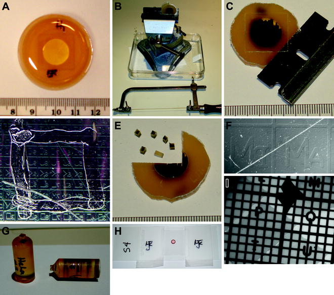
Fig. 2.

Sample handling and preparation steps, from embedding cells to imaging thin sections.

Mark the backside (the side opposite the cells attached to the coverglass) of the embedding plastic with a black permanent marker.

Place the chamber dish in the vise and use the jeweler’s saw to cut away the perimeter walls (Fig. 2b) (see Note 12).

Remove the walless chamber dish from the vise and use a safety razor blade to slide under the coverslip and remove it from the embedding resin (Fig. 2c) (see Note 13).

Once the coverglass is removed, examine the sample using a stereo microscope to check whether any remnants of the coverglass remain, and remove them with the razor blade.

With a permanent marker, trace the boundaries of the specific gridded area of the plastic containing the cells of interest (Fig. 2d).

Clamp the plastic disc in the vise, and with the jeweler’s saw cut out small ∼1.5 × 1.5 mm blocks from the area of the embedding plastic that contains the cells of interest (Fig. 2e).

Using forceps, place the individual blocks on a microscope slide with the cells side up, black marker side down.

Place the slide on the stage of the upright epifluorescence microscope and examine using the 10× Plan-Neofluar (N.A. 0.30) objective lens.

10.

Focus to the surface of the block using brightfield illumination.

11.

Double-check that the area of the coverslip grid containing the coordinates of interest is present in the block.

12.

Switch to epifluorescence illumination to check that the cells of interest survived the embedding and mounting within the individual blocks (see Note 14).

13.

Mark the name of the sample on the side of a pre-made Quetol “bullet” where the individual blocks will be mounted using 5 min epoxy glue (Fig. 2g).

14.

Mix equal parts of the 5 min epoxy glue and put a small drop on the top of the Quetol bullet using the wooden end of a cotton-tipped applicator.

15.

Using forceps, pick up the sides of the block to be mounted and place it in the drop of epoxy on top of the bullet, black side down. Avoid getting epoxy on the forceps.

16.

Use the wooden end of the cotton-tipped applicator to spread the epoxy onto the four side walls of the block, without spreading the epoxy on the top surface, to be sure it will be securely attached to the Quetol bullet once the epoxy hardens.

3.7 Sectioning the Mounted Blocks with an Ultramicrotome

Trim the block into a keystone shape using a safety razor blade.

The region of interest can be observed in the block when mounted in the ultramicrotome and can be rotated to provide optimal orientation for serial sectioning.

Obtain a ribbon of 5–15 serial ultrathin (50–70 nm) sections on the surface of the water in the diamond knife.

Manipulate the position of the ribbon of sections so that they are perpendicular to the parallel grid bars. As the ribbon is picked up, the region of interest should be carefully positioned so that it is not located over the grid bars (see Note 15).

Allow the grids to air dry and place in a grid holder box.

Although not strictly necessary, a thin (5 nm) carbon film can be applied to the specimen section using a Auto 306 evaporator. The thin carbon coating will help stabilize the sections under the electron beam in the EFTEM microscope.

3.8 Imaging the Thin Sections by Fluorescence Microscopy

Using clean forceps, place the grid on an ethanol-cleaned microscope slide with the sections on the top side away from the microscope slide.

Place a clean #1.5 coverslip over the grid.

Tape the left and right sides of the coverslip to the microscope slide to hold the coverslip in place (Fig. 2h).

Place a small drop of immersion oil on the coverslip and examine with the 63× Plan-apochromat (N.A. 1.4) objective lens on either the inverted or upright epifluorescence microscope.

Using brightfield illumination, focus on the grid and find the location of the sections (Fig. 2I) (see Note 16).

Adjust for optimal focus using epifluorescence excitation and acquire fluorescence images from the cells of interest (Fig. 3a, b) (see Note 17) (see Note 18).

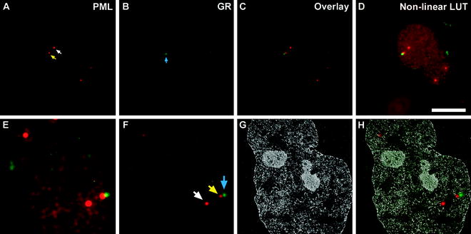
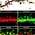
Fig. 3.

Aligning the fluorescence image map to the low magnification EFTEM image. Immunofluorescence images of PML ((a), red) and GR ((b), green) from ultrathin sections of double immunolabeled HeLa cells. The white arrow in (a) denotes one of the four PML bodies present in this ultrathin section, whereas, the yellow arrow denotes a PML body adjacent to the GR focus, denoted by the blue arrow in (b), as seen in the overlay image in (c). A nonlinear look-up table (Nonlinear LUT), with the brightness and contrast excessively adjusted for both the PML and GR intensities, to help display the boundary of the nucleus is shown in (d). A resized, rotationally transformed, and cropped version of the nonlinear LUT overlay image to match the magnification of the low magnification EFTEM image is shown in (e). The corresponding resized, rotationally transformed, and cropped but linearly adjusted (histogram stretched) overlay image is shown in (f). The colored arrows denote the same PML bodies as in (a) and GR focus as in (b). In (g), a low magnification (×7,000) net phosphorus EFTEM image of the same nucleus, with the fluorescence image overlaid on the net phosphorus image in (h). Scale bar, 10 μm.

Record the grid coordinates in the EM finder grids where the cells of interest are located, or the location of the serial sections on the grids.

Remove the grid from the microscope slide and place into a grid holder box.

With fluorescence images collected from the embedded and sectioned cells, using image processing software, such as MetaMorph or Adobe Photoshop, to adjust the brightness, contrast, and linearity (gamma) of the image intensity to exaggerate the low intensity pixels within the image and save as separate files (Fig. 3d). This nonlinear look-up table (LUT) will be useful as a guide to resize and align with images collected during EFTEM acquisition.

10.

The pixel size within both the fluorescence image and the EFTEM images, collected at different magnifications, should be known. The respective pixels can be used to calculate the difference in magnification between the fluorescence and EFTEM image(s) and either digitally zoom or resample the fluorescence image to use as an overlay mask on the acquired EFTEM image (see Note 19).

11.

Use the fluorescence image, adjusted with the nonlinear LUT, to view the boundaries of the nucleus and any structural clues to account for any differences in rotation between fluorescence image and the EFTEM image. The processed fluorescence image is used as a map to locate the position of the structures of interest within the EFTEM image (Fig. 3e) (see Note 20).

3.9 EFTEM Imaging of the Thin Sections

Stabilize the sections with a low flux of beam electrons at low magnification (see Note 21).

Check the alignment of the EFTEM microscope, including beam and energy selecting filter.

Acquire energy loss image series (one pre-edge and one post-edge image), with the energy selecting slit set at a width of 20 eV, for both phosphorus (L_II,III edge; pre-edge 120 eV and post-edge 155 eV) and nitrogen (N_K edge; pre-edge 385 eV and post-edge 415 eV) at different magnifications (7,000×, 12,000×, 30,000×, 50,000×, etc.). Frame the different regions of the nucleus containing the structures of interest, in this case, the PML bodies and GR focus (see Note 22).

The processed fluorescence image can be used as a map to help locate the subnuclear structures of interest within the energy loss images.

Steps 2 and 3 are repeated for each serial section containing the cell and subnuclear structures of interest.

3.10 Image Processing and Alignment of Fluorescence and EFTEM Images

Net elemental maps are generated from the EFTEM energy loss image series by dividing the respective element-enhanced post-edge image by the pre-edge image, using the Digital Micrograph EFTEM image acquisition and processing software (Fig. 4) (see Note 23).

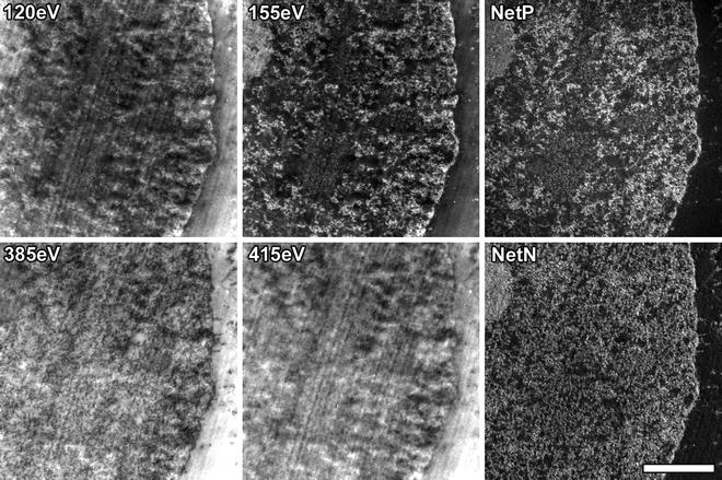
Fig. 4.

EFTEM energy loss image series and corresponding net element image maps. Pre-edge and post-edge images are collected for each specific element (120 eV and 155 eV, respectively, for phosphorus and 385 eV and 415 eV, respectively, for nitrogen) and the net element image map can be obtained by dividing the post-edge image by the pre-edge image. The raw images, without any contrast adjustment, collected at ×12,000 magnification are shown. Scale bar, 1.0 μm.

Linearly adjust the brightness and contrast (histogram stretch) for the EFTEM net elemental images and export them as TIFF files so that they can be arranged into figures using Adobe Photoshop.

The transformed (resized and rotated) and contrast-adjusted (histogram stretched) fluorescence image can be overlaid onto the low magnification (7,000×) EFTEM net phosphorus image (Fig. 5b).

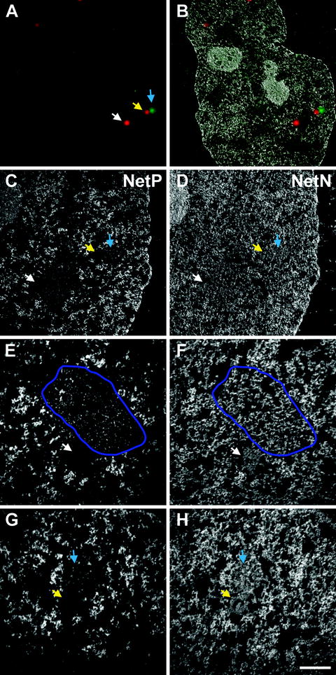
Fig. 5.

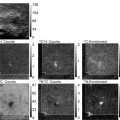
Net element EFTEM images of the ultrastructure of PML bodies, a glucocorticoid receptor focus and an interchromatin granule cluster. (a) The fluorescence overlay image acquired from the thin section, the white and yellow arrows denoting PML bodies and the blue arrow denoting the GR focus. An overlay of the fluorescence image with the low magnification (×7,000) net phosphorus EFTEM image is shown in (b). The higher magnification (×12,000) net phosphorus and net nitrogen image maps are shown in (c, d), respectively, with the arrows denoting the location of the PML bodies (white and yellow arrows) and GR focus (blue arrow). Even higher magnification (×30,000) net phosphorus (e, g) and net nitrogen (f, h) image maps of the two regions of the nucleus containing PML bodies are shown. In (e, f), the PML body (white arrow) is next to an interchromatin granule cluster (denoted by the encircling purple region of interest). The PML body contains very little phosphorus but considerable nitrogen ((compare (e) to (f)), whereas the IGC contains multiple RNP granules that provide signal in the phosphorus map (e). The PML body in (g, h) (yellow arrow) is beside the GR focus (blue arrow). Again, the PML body has very little phosphorus, but significant nitrogen signal, whereas the GR focus contains both phosphorus-rich fibrogranular structures as well as surrounding nitrogen signal. Scale bar, 500 nm.

Only gold members can continue reading. Log In or Register to continue