Detection and Labelling in Lumbar MR Images

Fig. 1

The task. Given a 3D MR lumbar spine image comprising of a stack of sagittal 2D slices as input (the mid-slice is shown on the left), localize and label in that image all the vertebrae that are present. The output (projected on the mid-slice on the right) consists of labelled tight bounding boxes around the vertebrae. Note that all the 2D slices in the 3D slice stack are searched for vertebrae candidates

In more detail, the input 3D image is a (sparsely spaced) stack of 2D sagittal images, and the output consists of labelled tight bounding boxes with labels around all the vertebrae in the image. Each bounding box is specified by its position, orientation, and scale. An example of the detection and labelling for a typical normal scan is shown in Fig. 1.

This detection task is challenging for a number of reasons, including: (1) the repetitive nature of the vertebrae, (2) varying image resolution and imaging protocols; artefacts, and (3) large anatomical and pathological variation, particularly in the lumbar spine. Various examples of challenging cases in our dataset are highlighted in Fig. 2. The anatomy and pathology variation can affect both the local vertebrae / disks appearance (e.g. degraded disks—Fig. 2h), and the global layout of the spine (e.g. scoliosis—Fig. 2c).

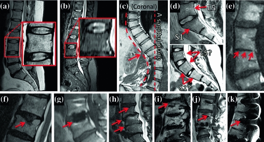
Fig. 2

Spine variation in our data. A collection of example images showing assorted image, anatomical and pathological modes of global variation of the spine shape, and local variation of the vertebrae, and the disks. Our algorithm is robust to all those variations. Abnormalities have been highlighted by the red arrows. a Normal spine with a zoom on a normal vertebra. b A low-resolution image. c A coronal view of a scoliotic spine, resulting in the spine not being cut by a single sagittal slice. d Top a normal sacrum, with unambiguous L5, S1 labelling based on shape and S1 and L5 orientation. Bottom a sacrum with ambiguous L5, S1 labelling based on their shape and orientation. e Joined vertebrae. f–j Pathologically deformed vertebrae and disks. k Magnetic susceptibility imaging artefacts

Contributions. Our method brings together two strong algorithms—the Deformable Part Model of Felzenszwalb et al. [1] based on Histogram of Oriented Gradients (HOG) image descriptors [10] and efficient inference on graphical models [11, 12]—making the algorithm accurate, robust, and efficient on challenging spine datasets. The algorithm is also tolerant to varying MR acquisition protocols, image resolutions, patient position, and varying slice spacing unlike related solutions in the literature. It localizes all the vertebrae present in a scan, and labels them correctly as long as the sacrum is present in the scan. Importantly, the method is appliccable to standard MRI protocols.

The method has two distinct stages. First, vertebrae candidates are detected by using a sliding window detector searching over position, scale, and angle (Sect. 2.1). Second, a graphical model is fitted to the set of candidate detections to find the optimal spine layout and labelling based on the unary SVM score of the detection for each part, and a spatial cost between each pair of connected parts (Sect. 2.2). The HOG descriptor captures the near rectangular shape of the vertebrae. We detect vertebrae rather than disks since the vertebrae shape is more consistent than the disk shape as the lumbar spine studies are more often aimed at targeting disk deformations, and more suitable to be modelled with HOG. Disk locations can easily be found after detecting vertebrae.

The closest previous work to ours is that of Oktay and Akgul [13]. They detect disks and vertebrae in the lumbar spine using a Pyramid HOG descriptor; however, they only detect six disks and vertebrae with their graphical model, require the existence of both T1 and T2 scans to first detect the spinal cord, and they have a separate HOG template for each vertebrae. In contrast, we demonstrate that just one generic vertebrae detector suffices for all vertebrae, and only require the T2 scan. Furthermore, they only use the mid-sagittal slices, making it only applicable to cases where all the spine parts are in the mid-sagittal slice, whereas we sequentially search for vertebrae in all the 2D images in the 3D stack (not restricted to the mid-sagittal slice).

Ghosh et al. [14] also use HOG features [10], however they do not label the vertebrae and make strong use of heuristics and information from complementary axial scans. They detect disks rather than vertebrae. Zhan et al. [15] present a robust hierarchical algorithm to detect and label arbitrary numbers of vertebrae and disks in nearly arbitrary field of view scans, as long as one of four ‘anchor’ vertebrae (C2, T1, L1, S) are present. They first detect the ‘anchor’ vertebrae, and then other ‘bundle’ vertebrae connected to it graphically. Although the method works very well within its domain, it requires isotropic 2.1 mm resolution scans which limits its applicability severely. Our method is not limited to this domain and, in particular, does not require the high isotropic resolution.

A further extensive body of literature on spine localization and labelling exists. In almost all the papers, the algorithms work in two stages. First, some anatomical parts characteristic of the spine are detected (vertebrae [16–18]/disks [14, 19–21]/both [13, 15]). Second, a spine layout model is fitted to the candidates to determine the best hypothesis for the spine layout. The spatial configuration of the spine parts, and in some cases also their individual characteristics [15, 18, 22], are taken into account to both label the disks and/or vertebra, and localize the spine.

2 Method

We present a method to localize and label vertebrae in lumbar MR images using two HOG-based detectors and a graphical model. First, given a stack of sagittal MR slices, vertebrae and sacrum candidates are detected using latent SVM on HOG in each slice as described in Sect. 2.1. Next, after local non-maxima suppression, the vertebrae candidates corresponding to the spine are picked and labelled by fitting a graphical model, as explained in Sect. 2.2.

2.1 Spine Part Detection

The spine part (vertebrae) detection is implemented using two detectors constituting latents SVMs on Histogram of Oriented Gradients (HOG) descriptors [10] using the Felzenszwalb VOC Challenge object detection framework [23]. We learn one generic 2D detector for vertebrae bodies (VBs), trained on all VBs in all the training images, and another more specific 2D detector for the sacrum, trained on the VBs of the first two links of the sacrum. Both the models are visualized along with a set of training samples in Fig. 3.

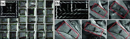
Fig. 3

The appearance model. Some training examples and a learned HOG template are shown for both the generic vertebrae body detector (a) and for the sacrum detector (b). The examples have been hand-annotated with tight Ground Truth bounding boxes as shown above and explained in Fig. 5

Training. Both the generic vertebrae body (VB) detector and the sacrum detector are trained using the Felzenszwalb detection framework [23]. The positive training examples for the VB detector are tight bounding boxes around the vertebral bodies of T10…L5 vertebrae with the bounding box sides parallel to the vertebral facets as shown in Fig. 3a. The positive training examples for the sacrum detector are tight bounding boxes around the first two links of the sacrum, with one side parallel to the posterior side of the sacrum as shown in Fig. 3b. The bounding boxes for both the VB and the sacrum are defined by fitting a minimum bounding rectangle to landmarks on them—four for the VB and eight for the sacrum. Each training sample is extracted from the slice cutting through the middle of the respective vertebral body.

For the VB detector, four HOG templates are trained, each of them of a different aspect ratio. The HOG templates are each 6 cells high, and 6, 7, 8, and 9 cells wide, corresponding to aspect ratios between 1 and 1.5. The HOG cell size for the VB model is $8 \times 8$ pixels. The HOG template for the sacrum detector is 9 cells high by 5 cells wide, with $8 \times 8$ pixel HOG cell size. The HOG feature vectors are 31-dimensional, with 18 contrast-sensitive, 9 contrast-insensitive direction bins; and 4 texture feature bins.

The HOG templates capture the rectangular shape of the vertebrae, with variations due to deformation, and the trapezoid shape of the first two links of the sacrum. The vertebrae show wide size and resolution variation and are all scaled and warped to match one of the aspect ratios at training. The model is learned iteratively in several steps, with new positive samples mined by running the detector on the positive samples, collecting the strongest detections as new positives, and training a new detector using the new positives.

The negative samples for the vertebrae detector are first picked randomly from mid-slices with a hand-drawn black polygon covering all the vertebral bodies. Next, an iterative learning procedure is employed to pick hard negatives as false positive detections on the negative training images as detailed in [23].

Testing. During the candidate detection step at test time, a previously unseen sagittal scan is taken as input, and tight bounding boxes around vertebrae candidates are returned as output. The candidate search is performed sequentially in all slices of the scan. The VB and sacrum detector are run on each slice of the scan, searching over position, scale, and angle, with the scan rotated by $-20^{\circ }$ to $20 ^{\circ }$ in $10^{\circ }$ increments. A feature pyramid is calculated for each angle, with HOG cells placed densely next to each other. The feature pyramid has 10 levels per doubling of resolution (10 levels per octave), with the image resized and resampled to 2 $\times$ the original size to 0.5 $\times$ the original size from the finest to coarsest scale. All the detections at all positions, scales, orientations are collected and transformed onto the original test image coordinate system as shown in Fig. 4.

Fig. 4

Vertebrae detection pipeline. a Input image. b All detections at all rotation angles and scales. The green rectangles are generic vertebrae, and the red rectangles are sacrum candidates. c All detections, with top detections shown in thick blue line, and the “ $$+$$