—true positives and  —true negatives) and incorrectly classified pixels (i.e.
  —false negatives and
  —false positives). Based on these values, the following ratios can be computed:
C.
Recall, also referred to as correct detection rate or true positive rate:  , i.e. the percentage of skin pixels correctly classified as skin [29].
 , i.e. the percentage of skin pixels correctly classified as skin [29].
D.
Precision:  , i.e. the percentage of correctly classified pixels out of all the pixels classified as skin [29].
 , i.e. the percentage of correctly classified pixels out of all the pixels classified as skin [29].
 ) [64], and the area under curve can also be used as the effectiveness determinant [69].
In our works we also investigated the false negative rate ( ) obtained for a fixed false positive error
  [46]. Furthermore, we used the minimal detection error (
 ), where the threshold is set to a value, for which this sum is the smallest. In this chapter we rely on false positive and false negative rate, and we present their dependence using
  curves, when it is applicable.
 ) obtained for a fixed false positive error
  [46]. Furthermore, we used the minimal detection error (
 ), where the threshold is set to a value, for which this sum is the smallest. In this chapter we rely on false positive and false negative rate, and we present their dependence using
  curves, when it is applicable.
3.2 Data Sets
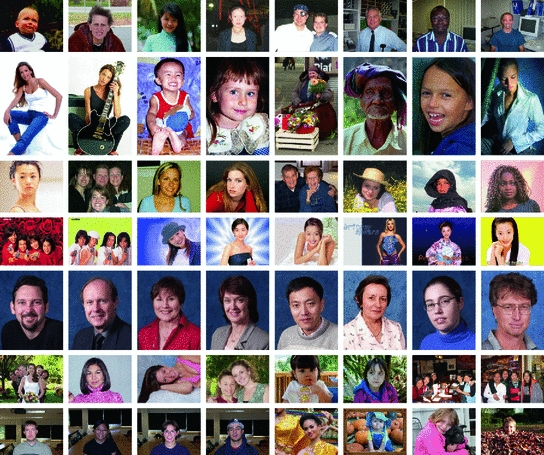
In their overview on skin color modeling, S.L. Phung et al. introduced a new benchmark data set, namely ECU face and skin detection database [64]. This data set consists of 4000 color images and ground-truth data, in which skin areas are annotated. The images were gathered from the Internet to provide appropriate diversity, and results obtained for this database were often reported in many works on skin detection. Therefore, this set was also used for all the comparisons presented in this chapter. Some examples of images from the data set are shown in Fig. 1. In all experiments reported here, the database was split into two equinumerous parts. The first 2000 images are used for training ( –
– ), and the remaining 2000 images are used for validation (
 –
– ). If an algorithm does not require training, then only the
  –
– set is used. The data set contains some images acquired in the same conditions, but as they appear close to each other in the data set, there is no risk that two similar images will repeat in
  –
– and
and  –
– .
.
 –
– ), and the remaining 2000 images are used for validation (
 –
– ). If an algorithm does not require training, then only the
  –
– set is used. The data set contains some images acquired in the same conditions, but as they appear close to each other in the data set, there is no risk that two similar images will repeat in
  –
– and
and  –
– .
.Among other data sets which can be used for evaluating skin detection, the following may be mentioned: (1) M.J. Jones and J.M. Rehg introduced the Compaq database [39], (2) S.J. Schmugge et al. composed a data set based on images derived from existing databases, in which they annotated skin regions [69], (3) we have created our hand image database for gesture recognition purposes (available at http://sun.aei.polsl.pl/~mkawulok/gestures) [46].
4 Skin Color Modeling
Classification of skin color modeling methods, which are given more attention in this section, is presented in Fig. 2, and several most important references are given for every category. In general, the decision rules can be defined explicitly in commonly used color spaces or in a modified color space, in which the skin could be easier separated from the background. Machine learning methods require a training set, from which the decision rules are learned. A number of learning schemes have been used for this purpose, and the most important categories are presented in the figure and outlined in the section.
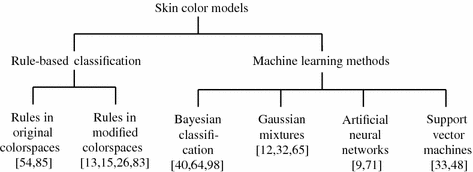

Fig. 2
General categories of skin color models
4.1 Color Spaces and Color Normalization
Skin color has been modeled in many color spaces using various techniques, which is summarized in Table 1. In many works it is proposed to reject the luminance component to achieve invariance to illuminance conditions. Hence, those color spaces are then preferred, in which the luminance is separated from the chrominance components, e.g.  ,
,  ,
,  . However, it was reported by many researchers that the illumination plays an important role in modeling the skin color and should not be excluded from the model [65, 72, 90]. The problem of determining an optimal color space for skin detection was addressed by A. Albiol et al., who provided a theoretical proof [5] that in every color space optimal skin detection rules can be defined. Following their argumentation, small differences in performance are attributed exclusively to the quantization of a color space. This conclusion is certainly correct, however the simplicity of the skin model may depend on the selection of color space. Based on the scatter analysis, as well as 2D and 3D skin-tone histograms, M.C. Shin et al. reported that it is the
  color space which provides the best separability between skin and non-skin color [72]. Furthermore, their study confirmed that the illumination is crucial for increasing the separability between the skin and non-skin pixels. In their later works, they argued that the
  color space should be chosen when the skin color is modeled based on the histogram analysis [69].
 ,
,  ,
,  . However, it was reported by many researchers that the illumination plays an important role in modeling the skin color and should not be excluded from the model [65, 72, 90]. The problem of determining an optimal color space for skin detection was addressed by A. Albiol et al., who provided a theoretical proof [5] that in every color space optimal skin detection rules can be defined. Following their argumentation, small differences in performance are attributed exclusively to the quantization of a color space. This conclusion is certainly correct, however the simplicity of the skin model may depend on the selection of color space. Based on the scatter analysis, as well as 2D and 3D skin-tone histograms, M.C. Shin et al. reported that it is the
  color space which provides the best separability between skin and non-skin color [72]. Furthermore, their study confirmed that the illumination is crucial for increasing the separability between the skin and non-skin pixels. In their later works, they argued that the
  color space should be chosen when the skin color is modeled based on the histogram analysis [69].
Color normalization plays an important role in skin color modeling [8, 53, 86]. M. Stoerring et al. investigated skin color appearance under different lighting conditions [79]. They have observed that location of the skin locus in the normalized  color space, where
  and
and  , depends on the color temperature of the light source. Negative influence of the changing lighting can be mitigated by appropriate color normalization. There exist many general techniques for color normalization [24, 25, 30, 58, 68], which can be applied prior to skin detection. Among them, the gray world transform is often reported as quite effective, while simple technique. Given an image with sufficient amount of color variations, the mean value of the
  ,
,  , and
, and  channels should average to a common gray value, which equals 128 in the case of the
  color space. In order to achieve this goal, each channel is scaled linearly:

where  indicates the channel (i.e.
  ,
,  or
or  ),
),  is the mean value in the channel for a given image prior to normalization, and
  is the value after normalization. In the modified gray world transform [24], the scale factors are determined in such a way that each color is counted only once for a given image, even if there are multiple pixels having the same position in the color space.
 color space, where
  and
and  , depends on the color temperature of the light source. Negative influence of the changing lighting can be mitigated by appropriate color normalization. There exist many general techniques for color normalization [24, 25, 30, 58, 68], which can be applied prior to skin detection. Among them, the gray world transform is often reported as quite effective, while simple technique. Given an image with sufficient amount of color variations, the mean value of the
  ,
,  , and
, and  channels should average to a common gray value, which equals 128 in the case of the
  color space. In order to achieve this goal, each channel is scaled linearly:
(1)
 indicates the channel (i.e.
  ,
,  or
or  ),
),  is the mean value in the channel for a given image prior to normalization, and
  is the value after normalization. In the modified gray world transform [24], the scale factors are determined in such a way that each color is counted only once for a given image, even if there are multiple pixels having the same position in the color space.
There are also a number of normalization techniques designed for the sake of skin detection. R.-L. Hsu et al. proposed a lighting compensation technique, which operates in  color space prior to applying an elliptical skin model [36]. The top 5 % of the gamma-corrected luminance values in the image define the reference white (
 , where
  and
and  are input and gamma-corrected luminance values, respectively). After that, the
  ,
,  and
and  components are linearly scaled, so that the average gray value of the reference-white pixels equals 255. This operation normalizes the white balance and makes the skin model applicable to various lighting conditions. P. Kakumanu [42] proposed to use a neural network to determine the normalization coefficients dynamically for every image. J. Yang et al. introduced a modified Gamma correction [91] which was reported to improve the results obtained using statistical methods. U. Yang et al. took into account the physics of the image acquisition process and proposed a learning scheme [93] which constructs an illumination-invariant color space based on a presented training set with annotated skin regions. The method operates in a modified
  color space. Skin pixels are subject to principal components analysis to determine the direction of the smallest variance. Thus, a single-dimensional space is learned, which minimizes the variance of the skin tone for a given training set.
 color space prior to applying an elliptical skin model [36]. The top 5 % of the gamma-corrected luminance values in the image define the reference white (
 , where
  and
and  are input and gamma-corrected luminance values, respectively). After that, the
  ,
,  and
and  components are linearly scaled, so that the average gray value of the reference-white pixels equals 255. This operation normalizes the white balance and makes the skin model applicable to various lighting conditions. P. Kakumanu [42] proposed to use a neural network to determine the normalization coefficients dynamically for every image. J. Yang et al. introduced a modified Gamma correction [91] which was reported to improve the results obtained using statistical methods. U. Yang et al. took into account the physics of the image acquisition process and proposed a learning scheme [93] which constructs an illumination-invariant color space based on a presented training set with annotated skin regions. The method operates in a modified
  color space. Skin pixels are subject to principal components analysis to determine the direction of the smallest variance. Thus, a single-dimensional space is learned, which minimizes the variance of the skin tone for a given training set.
4.2 Rule-Based Classification
Rule-based methods operate using a set of thresholds and conditions defined either in one of existing color spaces (e.g.  ) or the image is first transformed into a new color space, in which the skin color can be easier separated from the non-skin color. There have been a number of methods proposed which adopt such an approach and new algorithms are still being proposed. Unfortunately, the recent methods do not contribute much to the state of the art, which is confirmed by the presented experimental results.
 ) or the image is first transformed into a new color space, in which the skin color can be easier separated from the non-skin color. There have been a number of methods proposed which adopt such an approach and new algorithms are still being proposed. Unfortunately, the recent methods do not contribute much to the state of the art, which is confirmed by the presented experimental results.
One of the first skin color modeling techniques was proposed by K. Sobottka and I. Pitas in 1996. They observed that the skin tone can be defined using two ranges of ![$$S \in [0.23, 0.68]$$](/wp-content/uploads/2016/03/A308467_1_En_11_Chapter_IEq59.gif) and
and ![$$H \in [0, 50]$$](/wp-content/uploads/2016/03/A308467_1_En_11_Chapter_IEq60.gif) values in the
values in the  color model [74]. A modification of this simple technique was later proposed by S. Tsekeridou and I. Pitas [85] and it was used for face region segmentation in the image watermarking system [63]. The rule takes the following form in the
  color space:

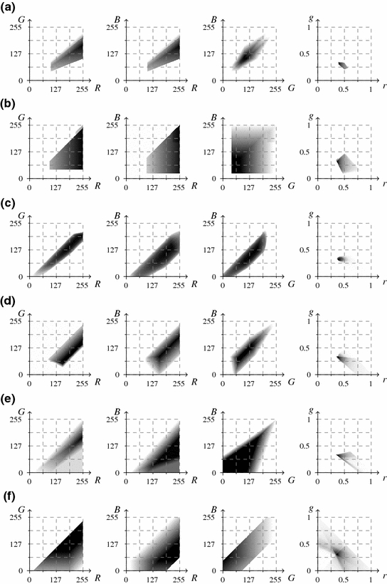
Projection of these rules onto the  color space is shown in Fig. 3a using
  ,
,  ,
,  and normalized
  planes. The darker shade indicates the higher density of skin pixels.
![$$S \in [0.23, 0.68]$$](/wp-content/uploads/2016/03/A308467_1_En_11_Chapter_IEq59.gif) and
and ![$$H \in [0, 50]$$](/wp-content/uploads/2016/03/A308467_1_En_11_Chapter_IEq60.gif) values in the
values in the  color model [74]. A modification of this simple technique was later proposed by S. Tsekeridou and I. Pitas [85] and it was used for face region segmentation in the image watermarking system [63]. The rule takes the following form in the
  color space:
(2)
 color space is shown in Fig. 3a using
  ,
,  ,
,  and normalized
  planes. The darker shade indicates the higher density of skin pixels.
J. Kovac et al. defined fixed rules [54, 76] that determine skin color in two color spaces, namely  and
and  (ignoring the luminance channel). The rules in
  are as follows:
![$$\begin{aligned} \left\{ \begin{array}{l} (R>95) \wedge (G>40) \wedge (B>20) \\ \max (R,G,B)-\min (R, G, B)>15 \\ \left| R – G \right| > 15 \wedge (R>G) \wedge (R>B)\\ \end{array} \right. \end{aligned}$$” src=”/wp-content/uploads/2016/03/A308467_1_En_11_Chapter_Equ3.gif”></DIV></DIV><br />
<DIV class=EquationNumber>(3)</DIV></DIV>for uniform daylight illumination or<br />
<DIV id=Equ4 class=Equation><br />
<DIV class=EquationContent><br />
<DIV class=MediaObject><IMG alt=]() 220) \wedge (G>210) \wedge (B>170) \\ \left| R – G \right| \le 15 \wedge (R>G) \wedge (R>B) \\ \end{array} \right. \end{aligned}$$” src=”/wp-content/uploads/2016/03/A308467_1_En_11_Chapter_Equ4.gif”>
220) \wedge (G>210) \wedge (B>170) \\ \left| R – G \right| \le 15 \wedge (R>G) \wedge (R>B) \\ \end{array} \right. \end{aligned}$$” src=”/wp-content/uploads/2016/03/A308467_1_En_11_Chapter_Equ4.gif”>
for flashlight lateral illumination. If the lighting conditions are unknown, then a pixel is considered as skin, if its color meets one of these two conditions. These rules are illustrated in  ,
,  ,
,  and
and  planes in Fig. 3b.
 and
and  (ignoring the luminance channel). The rules in
  are as follows:
(4)
 ,
,  ,
,  and
and  planes in Fig. 3b.
R.-L. Hsu et al. defined the skin model [36] in the  color space, which is applied after the normalization procedure outlined earlier in Sect. 4.1. The authors observed that the skin tone forms an elliptical cluster in the
  subspace. However, as the cluster’s location depends on the luminance, they proposed to nonlinearly modify the
  and
and  values depending on the luminance
  , if it is outside the range
 ![$$Y \in [125, 188]$$](/wp-content/uploads/2016/03/A308467_1_En_11_Chapter_IEq80.gif) . Afterwards, the skin cluster is modeled with an ellipse in the modified
. Afterwards, the skin cluster is modeled with an ellipse in the modified  subspace. Skin distribution modeled by these rules is presented in Fig. 3c.
 color space, which is applied after the normalization procedure outlined earlier in Sect. 4.1. The authors observed that the skin tone forms an elliptical cluster in the
  subspace. However, as the cluster’s location depends on the luminance, they proposed to nonlinearly modify the
  and
and  values depending on the luminance
  , if it is outside the range
 ![$$Y \in [125, 188]$$](/wp-content/uploads/2016/03/A308467_1_En_11_Chapter_IEq80.gif) . Afterwards, the skin cluster is modeled with an ellipse in the modified
. Afterwards, the skin cluster is modeled with an ellipse in the modified  subspace. Skin distribution modeled by these rules is presented in Fig. 3c.
Elliptical model of the skin cluster was also presented by J.-C. Terrillon et al., who argued that the skin color can be effectively modeled using the Mahalanobis distances computed in a modified  color space [83]. This model was further improved by F. Tomaz et al. [84].
 color space [83]. This model was further improved by F. Tomaz et al. [84].
G. Kukharev and A. Nowosielski defined the skin detection rules [57] using two color spaces, i.e.  and
and  . Here, a pixel value is regarded as skin:
Get Clinical Tree app for offline access
 and
and  . Here, a pixel value is regarded as skin:
In 2009, A. Cheddad et al. proposed to transform the normalized  color space into a single-dimensional error signal, in which the skin color can be modeled using a Gaussian curve [13]. After the transformation, a pixel is regarded as skin if it fits between two fixed thresholds determined based on the standard deviation of the curve. The model is also illustrated in the
  color space in Fig. 3e.
 color space into a single-dimensional error signal, in which the skin color can be modeled using a Gaussian curve [13]. After the transformation, a pixel is regarded as skin if it fits between two fixed thresholds determined based on the standard deviation of the curve. The model is also illustrated in the
  color space in Fig. 3e.
Recently, Y.-H. Chen et al. analyzed the distribution of skin color in a color space derived from the  model [15]. They observed that the skin color is clustered in a three-channel color space obtained by subtracting the
  values:
  . After that they set the thresholds in the new color space to classify every pixel. The rules are visualized in Fig. 3f.
 model [15]. They observed that the skin color is clustered in a three-channel color space obtained by subtracting the
  values:
  . After that they set the thresholds in the new color space to classify every pixel. The rules are visualized in Fig. 3f.
Fig. 4
Skin detection results obtained using different rule-based methods

Fig. 5
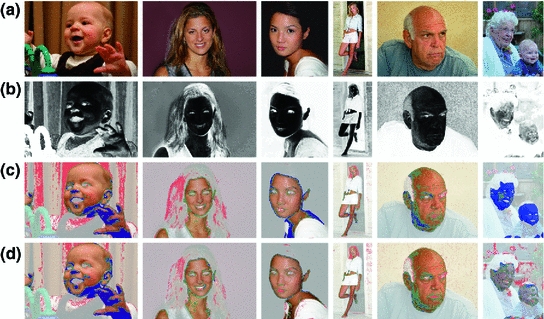
Skin detection results obtained using Bayesian classifier: original image (a), skin probability map (b), segmentation using a threshold optimized for the whole  –
– data set (c) and using the best threshold determined for each particular image (d)
 –
– data set (c) and using the best threshold determined for each particular image (d)
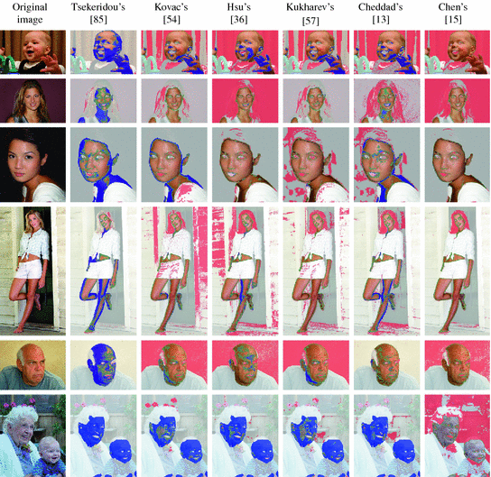
Some skin detection results obtained using six different methods are presented in Fig. 4. False positives are marked with a red shade, while false negatives—with the blue, and true positives are rendered normally. It can be seen from the figure that the detection error is generally quite high, however some methods present better performance in some specific cases. The overall performance scores are compared in Fig. 5. Rule-based models deliver worse results than the Bayesian skin model, however their main advantage lies in their simplicity. If the lighting conditions are controlled and fixed, then using a rule-based model may be a reasonable choice. Nevertheless, in a general case, the machine learning approaches outperform the models based on fixed rules defined in color spaces.
4.3 Machine Learning Methods
In contrast to the rule-based methods, the skin model can also be learned from a classified training set of skin and non-skin pixels using machine learning techniques. In most cases, such an approach delivers much better results and it does not require any prior knowledge concerning the camera characteristics or lighting conditions. It is often argued that the main advantage of the rule-based methods is that they do not require a training set. However, the rules are designed based on observed skin-tone distribution, which means that a form of a training set is required as well. J. Brand and J.S. Mason confirmed in their comparative study that the histogram-based approach to skin modeling outperforms the methods which operate using fixed thresholds in the  color space [11]. Some machine learning techniques require large amount of training data (e.g. Bayesian classifier), while others are capable of learning effectively from small, but representative training sets. In this section the most important machine learning techniques used for skin detection are presented and discussed.
 color space [11]. Some machine learning techniques require large amount of training data (e.g. Bayesian classifier), while others are capable of learning effectively from small, but representative training sets. In this section the most important machine learning techniques used for skin detection are presented and discussed.
4.3.1 Bayesian Classifier
Analysis of skin and non-skin color distribution is the basis for many skin detection methods. They may consist in a simple analysis of 2D or 3D histograms of skin color acquired from a training set or may involve the Bayesian theory to determine the probability of observing the skin given a particular color value. Such an approach was adapted by B.D. Zarit et al., whose work [98] was focused on the analysis of the skin and non-skin histograms in two-dimensional color spaces. At the same time, M.J. Jones and J.M. Rehg proposed to train the Bayesian classifier in the  space using all three components [39, 40]. The main principles of these techniques are as follows.
 space using all three components [39, 40]. The main principles of these techniques are as follows.
At first, based on a training set, histograms for the skin ( ) and non-skin (
 ) classes are built. The probability of observing a given color value (
 ) in the
  class can be computed from the histogram:

where  is the number of
  -colored pixels in the class
  and
and  is the total number of pixels in that class. Maximal number of histogram bins depends on the pixel bit-depth and for most color spaces it equals
  . However, it is often reported beneficial to reduce the number of bins per channel. Our experiments, reported later in this section, indicated that the optimal histogram bin number depends on the training set size. Basically, the smaller the training set, the smaller number of bins should be used to achieve higher generalization.
 ) and non-skin (
 ) classes are built. The probability of observing a given color value (
 ) in the
  class can be computed from the histogram:
(6)
 is the number of
  -colored pixels in the class
  and
and  is the total number of pixels in that class. Maximal number of histogram bins depends on the pixel bit-depth and for most color spaces it equals
  . However, it is often reported beneficial to reduce the number of bins per channel. Our experiments, reported later in this section, indicated that the optimal histogram bin number depends on the training set size. Basically, the smaller the training set, the smaller number of bins should be used to achieve higher generalization.
It may be expected that a pixel presents the skin, if its color value has a high density in the skin histogram. Moreover, the chances for that are larger, if the pixel’s color is not very frequent among the non-skin pixels. Taking this into account, the probability that a given pixel value belongs to the skin class is computed using the Bayes rule:

where a priori probabilities  and
and  may be estimated based on the number of pixels in both classes, but very often it is assumed that they both equal
  . If the training set is large enough, then the probabilities
  for all possible color values can be determined, and the whole color domain is densely covered. For smaller training sets, the number of histogram bins should be decreased to provide proper representation for every bin. The learning phase consists in creating the skin color probability look-up table (
 ), which maps every color value in the color space domain into the skin probability (which is also termed as skinness). After training, using the look-up table, an input image is converted into a skin probability map, in which skin regions may be segmented based on an acceptance threshold (
 ). The threshold value should be set to provide the best balance between the false positives and false negatives, which may depend on a specific application. This problem is further discussed in Sect. 7.

(7)
 and
and  may be estimated based on the number of pixels in both classes, but very often it is assumed that they both equal
  . If the training set is large enough, then the probabilities
  for all possible color values can be determined, and the whole color domain is densely covered. For smaller training sets, the number of histogram bins should be decreased to provide proper representation for every bin. The learning phase consists in creating the skin color probability look-up table (
 ), which maps every color value in the color space domain into the skin probability (which is also termed as skinness). After training, using the look-up table, an input image is converted into a skin probability map, in which skin regions may be segmented based on an acceptance threshold (
 ). The threshold value should be set to provide the best balance between the false positives and false negatives, which may depend on a specific application. This problem is further discussed in Sect. 7.
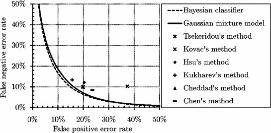
Fig. 6
 curves obtained for the Bayesian classifier and the Gaussian mixture model, and errors obtained for the rule-based skin detectors
 curves obtained for the Bayesian classifier and the Gaussian mixture model, and errors obtained for the rule-based skin detectors
Examples of the skin segmentation outcome obtained using the Bayesian classifier are presented in Fig. 6. Original images (a) are transformed into skin probability maps (b) which are segmented using two threshold values, namely globally (c) and locally (d) optimized. The former is set, so as to minimize the detection error for the whole data set, while the latter minimizes the error independently for each image. It can be noticed that the detection errors are smaller than in case of using the rule-based methods, whose results were shown in Fig. 4. The advantage is also illustrated in Fig. 5 in a form of  curves. Here, the results obtained for the rule-based methods are presented as points, because their performance does not depend on the acceptance threshold. In the case of the Bayesian classifier, as well as the Gaussian mixture model, which is discussed later in this section, skin probability maps are generated, hence the
  curves may be rendered. It can be seen that the Bayesian classifier outperforms the rule-based methods and also it is slightly better than the Gaussian mixture model.
 curves. Here, the results obtained for the rule-based methods are presented as points, because their performance does not depend on the acceptance threshold. In the case of the Bayesian classifier, as well as the Gaussian mixture model, which is discussed later in this section, skin probability maps are generated, hence the
  curves may be rendered. It can be seen that the Bayesian classifier outperforms the rule-based methods and also it is slightly better than the Gaussian mixture model.
4.3.2 Gaussian Mixture Models
Using non-parametric techniques, such as those based on the histogram distributions, the skin probability can be effectively estimated from the training data, providing that the representation of skin and non-skin pixels is sufficiently dense in the skin color space. This condition is not necessarily fulfilled in all situations. A technique which may be applied to address this shortcoming, consists in modeling the skin color using a Gaussian mixture model (GMM). Basically, if the histogram is approximated with a mixture of Gaussians, then it is smoothed at the same time, which is particularly important in case of sparse representation. GMM has been used for skin detection in various color spaces, in which a single pixel is represented by a vector  of the dimensionality
  , whose value depends on a particular color space. Usually
  or
or  , but also skin color was modeled using Gaussians in the one-dimensional spaces [13, 94].
 of the dimensionality
  , whose value depends on a particular color space. Usually
  or
or  , but also skin color was modeled using Gaussians in the one-dimensional spaces [13, 94].
In general, using the adaptive Gaussian mixture model, the data are modeled with a mixture of  Gaussian distributions. In the majority of approaches, only the skin-colored pixels are modeled with the Gaussian mixtures, nevertheless non-skin color could also be modeled separately. Thus, in such situations, these two models (i.e. skin and non-skin) are created. Each Gaussian distribution function is characterized with a weight
  . The probability density function of an observation pixel
  in the mixture model is given as:

where  is the probability for a single Gaussian:

Here,  is the
  th Gaussian weight estimation and
  is the parameter vector of a mixture composition.
  consists of
  th Gaussian distribution parameters, that is, the mean value
  and covariance
  , which is a
  positive definite matrix. The parameters of GMM are estimated based on the expectation-maximization (EM) algorithm.
 Gaussian distributions. In the majority of approaches, only the skin-colored pixels are modeled with the Gaussian mixtures, nevertheless non-skin color could also be modeled separately. Thus, in such situations, these two models (i.e. skin and non-skin) are created. Each Gaussian distribution function is characterized with a weight
  . The probability density function of an observation pixel
  in the mixture model is given as:
(8)
 is the probability for a single Gaussian:
(9)
 is the
  th Gaussian weight estimation and
  is the parameter vector of a mixture composition.
  consists of
  th Gaussian distribution parameters, that is, the mean value
  and covariance
  , which is a
  positive definite matrix. The parameters of GMM are estimated based on the expectation-maximization (EM) algorithm.
The EM algorithm is an iterative method for finding the maximum likelihood (ML) function:

This function estimates the values of the model parameters, so as they best describe the sample data.

(10)
The EM algorithm includes two steps, namely:
Expectation: Calculate the expected value of the log likelihood function:
![$$\begin{aligned} Q(\varTheta |\varTheta ^{(t)}) = E \left[ \log \mathcal {L}(\mathbf {X};\varTheta ) \big | \mathbf {X},\varTheta ^{(t)} \right] , \end{aligned}$$](/wp-content/uploads/2016/03/A308467_1_En_11_Chapter_Equ11.gif)
where  is the current set of the parameters.
![$$\begin{aligned} Q(\varTheta |\varTheta ^{(t)}) = E \left[ \log \mathcal {L}(\mathbf {X};\varTheta ) \big | \mathbf {X},\varTheta ^{(t)} \right] , \end{aligned}$$](/wp-content/uploads/2016/03/A308467_1_En_11_Chapter_Equ11.gif)
(11)
 is the current set of the parameters.
Maximization: Find the parameter that maximizes this quality:

In this algorithm, the GMM parameters are determined as follows:


The EM algorithm is initiated with a given number of Gaussian mixtures ( ) and the model parameters are obtained using the
  -means algorithm.

(12)

(13)

(14)

(15)

(16)
 ) and the model parameters are obtained using the
  -means algorithm.
As mentioned earlier, skin color has been modeled using GMM in various color spaces. Normalized  chromaticity space (i.e.
 ![$$\mathbf {x}=[r, g]^T$$](/wp-content/uploads/2016/03/A308467_1_En_11_Chapter_IEq137.gif)


 chromaticity space (i.e.
 ![$$\mathbf {x}=[r, g]^T$$](/wp-content/uploads/2016/03/A308467_1_En_11_Chapter_IEq137.gif)
Stay updated, free articles. Join our Telegram channel

Full access? Get Clinical Tree


